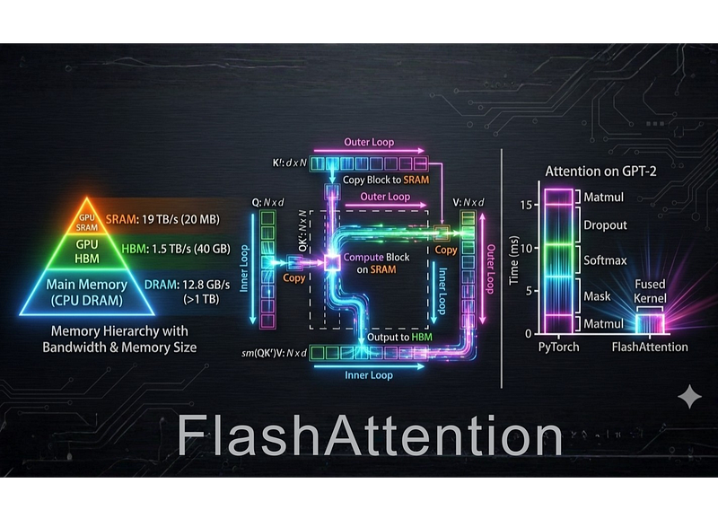
In the summer of 2022, when the world was still reeling under the effects of COVID, researchers Tri Dao and Dan Fu, while working at Stanford University, were grappling with a tough problem: the attention mechanism in transformers was becoming a computational bottleneck. As language models grew larger and sequences grew longer, the quadratic memory complexity of standard attention was proving unsustainable. Training and inference were painfully slow, and the promise of truly long-context language models seemed out of reach.
People tried various methods where they changed the nature of the attention calculations basically to reduce the complexity of the underlying calculations. They were thinking if too many calculations are taking place, can I somehow reduce the scope of the calculations. Sparse attention patterns like Longformer selectively masked out certain token interactions. Low-rank approximations like Performer used clever mathematical tricks to compress the attention matrix. Linear attention reformulated the computation order entirely. But these approaches generally resulted in some speed improvements while sacrificing accuracy — the approximations and modifications meant models couldn’t capture the full richness of attention patterns that made transformers so powerful in the first place.
The fundamental trade-off seemed unavoidable: you could have speed, or you could have accuracy, but not both.
 Dan Fu (left) and Tri Dao (right)
Interestingly, this turned out to be a mirage. There was a third dimension which people were not considering, and hence they were facing this supposed wall. The trade-off between speed and accuracy wasn’t fundamental. It was just an artifact of how everyone was thinking about the problem.
In this post, we’ll talk about this third dimension and how Flash Attention solved the problem in a very interesting manner. Flash Attention was able to unlock a power boost that propelled the field of AI into another level of gameplay (I hope I am not stretching the gaming metaphor too much). The moral of the story is that many times what we think of as a bottleneck may not really exist. You just might not be looking at the problem from the right angle.
GPUs and Memory Bounded Algorithms#
It's common knowledge that if you want to run deep learning models fast, you need to run on them on the GPU. But what exactly is the GPU.
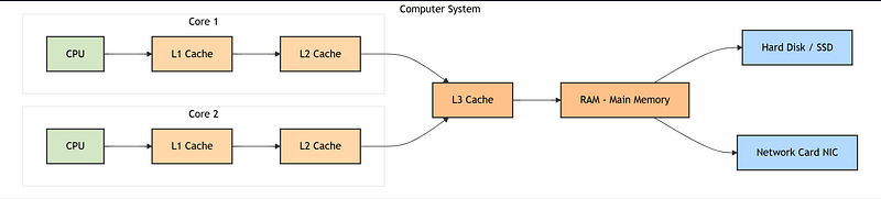 fig1: CPU cache hierarchy
A good way of understanding the GPU is to contrast it with the CPU. You want to run fast applications, so maybe you start with the biggest core and plug in the biggest memory to it. But a big memory can be slow to access, so you put in multiple hierarchies of caches in between such as L1, L2 and L3 caches.
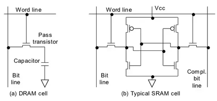 fig2: DRAM and SRAM. source
Now you might ask, how are caches better than main memory if both are memory. There are various reasons for this. Caches are static RAM (SRAM) and main memory is dynamic RAM (DRAM). SRAM is and can be considerably faster than DRAM the values are kept statically so they don't have to be refreshed which takes away cycles. DRAM is dynamic, like tiny rechargeable batteries, you have to regularly recharge the ones so they don't drain away and become zeros. This steals cycle time in addition to how you have to access the bits, etc. Being on the same die as or nearer the processor reduces the round trip, both L1 and L2 are faster than DRAM from an access perspective. Read more here, here and here.
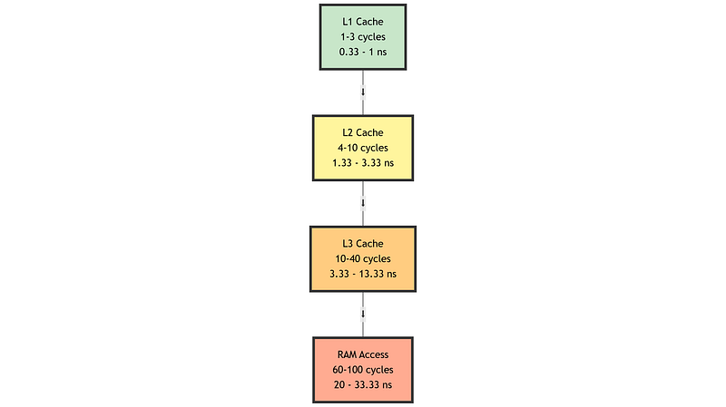 fig3: diagram by author
Why do we need multiple levels then? We need cache hierarchy because we are fundamentally constrained by the physical relationship between size and speed on the die. Each cache bit requires transistors, and communication speed degrades with distance due to substrate impedance and complex quantum phenomena, creating a trade-off where larger caches must be positioned farther from processing units like the MMU and ALU. A single large cache near all subunits simultaneously is impractical because it would consume excessive space and force the subunits themselves farther apart, degrading their inter-communication. Instead, processor designers implement a tiered approach: L1 caches are kept small and extremely close to their respective cores for maximum speed, L2 caches provide moderate capacity with slightly reduced locality, and in multicore systems, a shared L3 cache sits between cores offering substantial storage with reasonable access times for all cores. When data is needed, the processor searches sequentially through L1, L2, and L3 before accessing slower system memory, then propagates the fetched data back up through the cache hierarchy. This is just a simple explanation though. The actual cache management mechanisms in modern processors involve considerably more sophisticated protocols which is outside the scope for this blog post.
While discussing CPUs we digressed a little bit into caches as well, but this will be apparent in some time. The important thing to note is that each CPU gets a sophisticated memory management system.
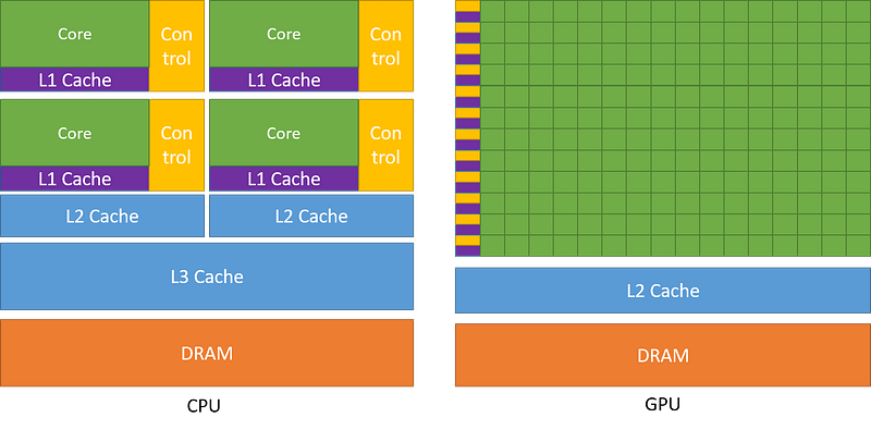 fig4: source: docs.nvidia.com
Now if you want to scale from couple of cores, to thousands of cores so that you can scale up the computations, there are couple of choices that you have to make. You should reduce the amout of control logic you have per core. This also means that you cannot support the huge amount of caches dedicated to the cores. Just because the number of cores is huge now, the cache placement and wiring becomes untenable. Else your machine will become too costly, and you will not be able to sell them on the market. The CPU cores are too big; they are quite general purpose so you can reduce the amount number of operations they can handle. You can see the instructions in the x86 architecture.
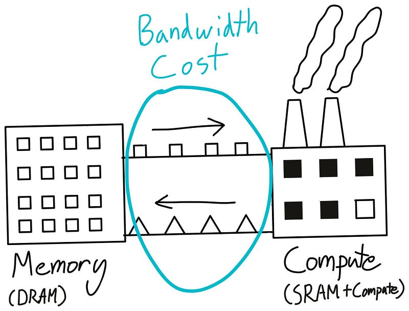 fig5: source: horace.io
All this discussion of cores and caches brings us to the difference between compute bounded and memory bounded in terms of algorithms. You can double the number of cores in your GPUs, but that does not ensure that your algorithm will run 2x. For example, let's say you want to run torch.sin it would mean transferring the vector from cpu memory to GPU memory DRAM, which we can call the High Bandwidth Memory (HBM), then transfer to the registers and then doing the actual computation. Once the computation is done, you will transfer it back to the HBM. If there are further computations, then you can keep it in the HBM or else you will need to move it to the CPU for IO operations. All these moving data back and forth means that it does not matter if your computations are fast, if your transferring is slow your overall latency is slow. For more explanation, please go through this amazing blog regarding this issue.
So, what does this have to do with attention. Let's go over the standard attention mechanism and understand the core challenge of attention with respect to the GPU.
Standard Attention Recap#
Above is the standard attention equation that is used to compute the attention scores in most transformer modules. So we can see that we can write the above equation 1 in terms of the below algorithm.
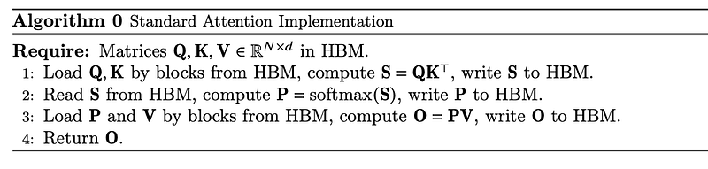 fig 6: standard attention algorithm, mentioned in arxiv.org/abs/2205.14135
The implementation is written in this way to highlight the amount of memory reads and writes that is done. Thus, your attention calculation is a combination of both computation and the data transfers in memory. If your computation is fast but your memory transfers are slow, your overall calculations would be slower.
Matrix Multiplication using Tiling and Recomputation#
Before moving ahead and explore the core algorithm of flash attention, we will need to wrap our heads around two concepts — tiling and operator fusion. In literature and various blog posts, you may come across the terms shared memory and global memory. This is the same as the caches and the SRAM or HBM memory that we have earlier. The caches are called shared memory because the cores don't get dedicated memories like CPU cores get. I will discuss the memory layouts for the GPU in more detail in a later blog post. The meat is that shared memory is fast but small. Hence if we want to use some values frequently then it better if we can somehow fit them into the shared memory instead of relying on global memory. This strategy is called Tiling.
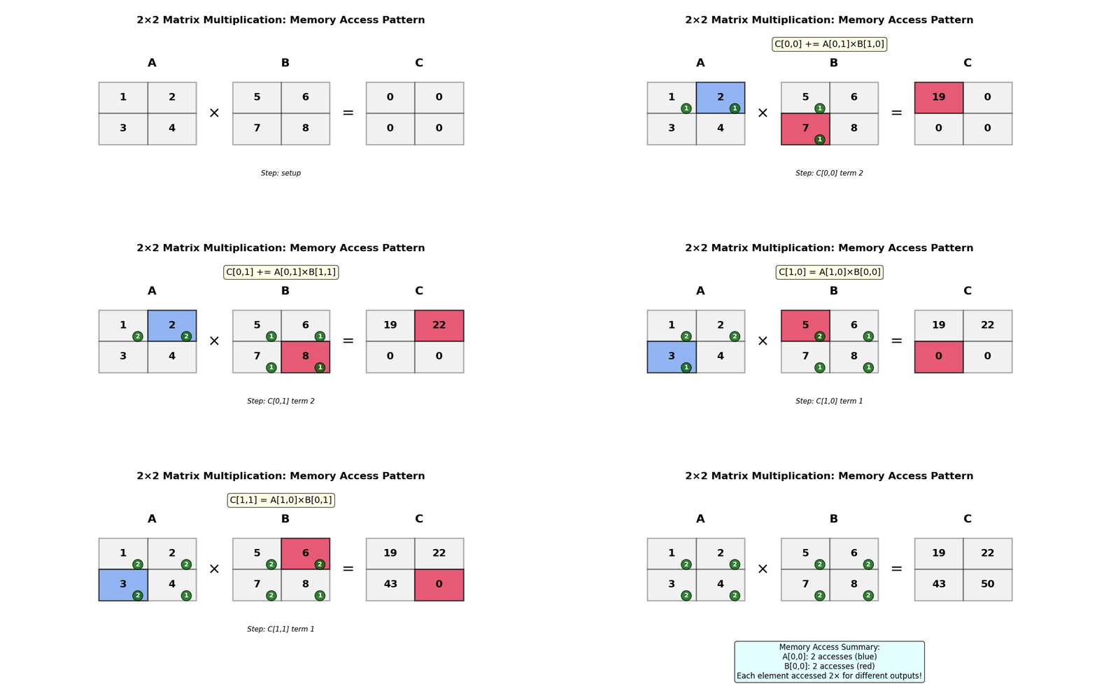 fig 7: matrix multiplication pattern for 2x2 matrix
Lets first go over matrix multiplication by taking the simplest case of a 2x2 matrix multiplication C = AB. In the above example, to compute the first element in the output C: 19 = A00 * B00 + A01 * B10 = 1 x 5 + 2 * 7. In this way you can fill up the rest of the elements in matrix C. Observe that to compute each element in C, you will need to access each element in the input matrices twice. If the program needs to repeatedly access the global memory for each cell computation, then it will be slow. Instead, if we load the matrices A and B into the shared memory, then each element will need to be accessed once from the global memory. The subsequent call can be done from the shared memory itself. Observe that if you generalize this to n elements, the number of memory accesses scale to 2n for the naive case. Hence the savings in terms of memory go from 2n to just 2 from the global memory. Please go over this blog post for better clarity.
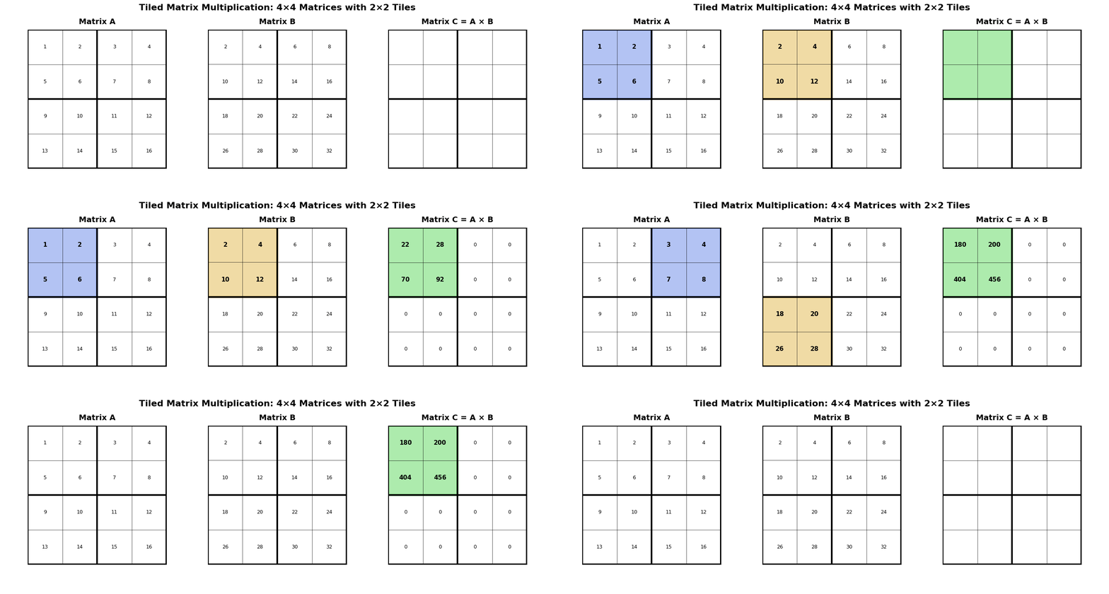 fig 8: gif by author; generated in colab
What if your matrices A and B are too big to fit into the shared memory. You can divide the matrix into blocks of size block size x block size (BSxBS) that can be fit into memory and then proceed with the computation. For our understanding and to keep the math simple let the dimensions for all A, B and C matrices be NxN. Notice that during the computation of matrix C, the result is just a partial sum; so, for the final result all the dot products need to be accumulated into a final sum. Notice that to compute each block in output C you needed to K = N/BS iterations. Total iterations for entire C matrix: \(K\times K\) blocks \(\times\) K iterations per block = \(K^3\) iterations. During each tile computation there are 2BSxBS memory operations. This gives us a total of \(2K^3\times BS^2\) = \(2N^3/BS\) memory operations. Without tiling, we would need approximately \(2N^3\) memory operations with each element loaded multiple times from slow global memory. With tiling, we achieve a \(BS\times\) reduction in memory bandwidth by loading each tile once into fast shared memory and reusing it across multiple computations. This is why tiling is fundamental to efficient GPU matrix multiplication.
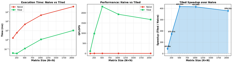 fig 9: performance comparison
Code 1
======================================================================
DETAILED COMPARISON: NAIVE vs TILED
======================================================================
    Size |   Naive (ms) |   Tiled (ms) |    Speedup |  Improvement
----------------------------------------------------------------------
 128×128  |       1.5895 |       0.0369 |      43.08x |        97.7%
 256×256  |       5.9405 |       0.0343 |     173.27x |        99.4%
 512×512  |      48.3408 |       0.1162 |     415.92x |        99.8%
1024×1024 |     460.5318 |       1.1129 |     413.80x |        99.8%
2048×2048 |    3888.4189 |      10.2782 |     378.32x |        99.7%
======================================================================
But just the theoretical understanding is not enough. How fast is the tiled logic in practice? I wrote a benchmarking script between naive matrix multiplication and tiled matrix multiplication and run it on colab which gave me a Tesla T4 GPU in the free tier. You can go through the code in this link. The code is in triton-lang which is a popular paradigm for writing efficient GPU code. You can see for current LLM matrix multiplication with sizes of 2048, the performance improvement is 378x. Disclaimer: The code is for educational purposes will still be slower than pytorch because pytorch uses highly optimised gemm modules.
 fig 10: source: giphy.com
Why Tiling Works.Tiling leverages several principles of computer architecture:
- Data Locality: It ensures that data being actively used by the processor stays in the fastest available memory (cache/shared memory), maximizing data reuse.
- Parallelization: The operations on different tiles of the resulting matrix can often be computed independently and in parallel across multiple processor cores or GPU threads.
- Vectorization: Tiled operations are often designed to be compatible with Single Instruction, Multiple Data (SIMD) instructions, allowing a single processor core to perform multiple operations simultaneously.
The result is a substantial reduction in memory access time and an increase in overall computational speed and efficiency. So, if we have some complex operations, we should look forward to applying tiling as much as possible. Basically, utilize all our strengths and bring as much grocery as needed in one trip.
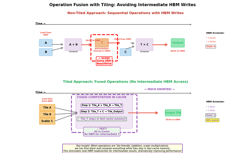 fig 11: Operation fusion with Tiling
Two or more matrices can be tiled, and the final output can be calculated in one go. Basic matrix operations such as addition and scalar multiplication are tile friendly. If two or more operations are tile friendly, then you can combine them to compute all the operations in an online manner. The advantage is that you won't need to write the intermediate results to HBM, thus getting a speed up in the overall operation.
The Softmax Conundrum#
Based on the formula in equation 1, the attention is implemented as shown in equations 2–6. First, we calculate QKT and multiply with a scaling factor \(\tau\). This scaling factor \(\tau\) is generally realized as \(1/\sqrt{d}\) but can be something else as well. Then we apply a mask function in equation 3, that sets some entries in the input to \(-\infty\) and other entries are the same. Then dropout is applied element wise. This means that if your dropout probability is p, then some outputs are marked 0 with probability p and others are scaled down (x/(1-p)). Lastly this output is multiplied with V matrix. The outputs of equations 2–5 are in NxN matrices while for equation 6 we get Nxd dimensions as the output.
In the above equations, equation 2 and 3 can be fused and equation 5 and 6 can be fused. But the softmax is different. There is a fundamental incompatibility between the global nature of the softmax function and the tiling strategy to fit large attention matrix into the fast GPU SRAM memory. Notice from the softmax equation 7, you need to know the global sum of all the values in the row to ensure the proper normalization. But in the tiling strategy discussed above, you only have access to a small block (tile) of a row, you cannot know the global statistics for the entire row until you have seen all the tiles. This is a crucial problem that flash attention solves.
Code 2
import numpy as np

def naive_softmax(x):
    """Naive softmax - numerically unstable!"""
    exp_x = np.exp(x)
    return exp_x / np.sum(exp_x)

x = np.array([1000.0, 1001.0, 1002.0])
result = naive_softmax(x)
print(f"\nResult: {result}")

Output: Result: [nan nan nan]
Code 2: naive softmax in NumPy — large values overflow to NaN
If we try to make some modifications in the softmax calculation in equation 7, we need to keep in mind another issue with the formula. The equation puts a strain on the maximum range our floating point values can hold. The maximum value for float16 representation is 65504, so if the value of x is greater than 11, there will be an overflow and our calculations will be wrong and we will get nans. This is shown in Code 2 above and you can try the full example in the colab code here.
To get around this fact, we generally find the maximum value of our tensor and subtract this from the exponent. This makes sure that the sum in the denominator is never greater than the floating point can hold. Doing this is equivalent to the softmax equation 7 as shown in the derivation above. It's just a multiplication of 1/e^m on both the numerator and the denominator.
Safe Softmax Algorithm#
If we implement the above changes, we get the below implementation (Code 3).
Code 3
import numpy as np

def safe_softmax_3pass(x):
    """
    3-pass safe softmax algorithm as described in FlashAttention paper.

    Pass 1: Compute maximum value m_i = max(x)
    Pass 2: Compute denominator d_i = sum(exp(x_j - m_N))
    Pass 3: Compute final softmax a_i = exp(x_i - m_N) / d_N
    """
    # Pass 1: Find maximum
    m = -np.inf
    for i in range(len(x)):
        m = max(m, x[i])

    # Pass 2: Compute denominator
    d = 0.0
    for i in range(len(x)):
        d = d + np.exp(x[i] - m)

    # Pass 3: Compute final softmax values
    a = np.zeros_like(x)
    for i in range(len(x)):
        a[i] = np.exp(x[i] - m) / d

    return a
Code 3: safe 3-pass softmax — subtract the row maximum for stability
In Code 3, we go over the values and find the maximum value, then we go over the values again to compute the sum of the discounted exponentials and then finally we compute the softmax values. You can check the correctness of this algorithm programmatically as well in this colab link.
Thus there are 3 iterations to computing the softmax values. This creates repeated access of the HBM memory, which is a massive problem as we have discussed before. We want to reduce this repeated back and forth from the HBM memory. In the flash attention paper, the authors worked out a method to reduce this algorithm to a single pass algorithm and fused it with the other operations in attention.
Online Softmax#
 Natalia Gimelshein (left) and Maxim Milakov (right)
To fix the repeated HBM memory issue in safe softmax, Maxim Milakov and Natalia Gimelshien came up with the online softmax algorithm (paper link) in 2018 while working at NVIDIA. In this they found a way to compute the maximum and the normalization factor together.
In the safe softmax equation 8, if the denominator sequence is given by \(\ell_i\) (as per the notation in the flash attention paper), then we can define the denominator sequence as the sum of the exponentials discounted by the overall maximum value as shown in equation 9. We want to remove that dependency on N in this equation. For this lets create a surrogate sequence \(\ell’_i\) as shown in equation 10 where we replace \(m_N\) with the current maximum seen so far \(m_i\). This implies that the final \(\ell_N\) is the same as \(\ell’_N\) when the computation for the full vector sequence is complete. This enables us to find a recurrence relation between \(\ell’_i\) and \(\ell’_{i-1}\) as seen in below derivation.
In the above derivation, in equation 12, we take eq10 and take out the final element. Eq13 and 14 are simple algebraic manipulation, make sure you understand it. Finally in equation 15 we arrive at a recurrence relation between \(\ell'_i\) and \(\ell'_{i-1}\). This rescaling adjusts the previously accumulated denominator whenever the maximum changes, ensuring that \(\ell'_i\) always represents \(\sum_{j=1}^{i} \exp(x_j - m_i)\). Notice that the dependency is only on current max \(m_i\) and previous max \(m_{i-1}\). This enables us to compute \(m_j\) and \(\ell'_j\) which are the full sequence within the same for loop. This means that now we can fuse pass1 and pass2 shown in the 3-pass solution into a single loop as shown below (Code 4).
Code 4
def softmax_2pass(x):
    """
    2-pass online softmax algorithm.

    Pass 1 (online): Update both m_i and l_i together
        m_i = max(m_{i-1}, x_i)
        l'_i = l'_{i-1} * exp(m_{i-1} - m_i) + exp(x_i - m_i)
    Pass 2: Compute final softmax values
        a_i = exp(x_i - m_N) / l'_N
    """
    N = len(x)

    # Pass 1: Online update of max and denominator
    m = -np.inf
    l_prime = 0.0

    for i in range(N):
        m_prev = m
        m = max(m_prev, x[i])
        # Rescale previous denominator and add new term
        l_prime = l_prime * np.exp(m_prev - m) + np.exp(x[i] - m)

    # Pass 2: Compute final softmax values
    a = np.zeros_like(x)
    for i in range(N):
        a[i] = np.exp(x[i] - m) / l_prime

    return a
Code 4: fused two-pass online softmax — running max and denominator in one loop
Go through Code 4, the algorithm shown above. Notice that the current max \(m_i\) and \(\ell _i\) are computed within a single for loop. The l_prime value is in accordance with the relation derived in eq15. The correctness comparison between the two algorithms is shown in this colab link. However, we still need to compute the softmax in 2 passes. So the obvious question is can we now reduce to a single pass to minimise global I/O?
Flash Attention#
The answer to the above question is unfortunately NO, but keep in mind that we don't really require the softmax output. The intermediate outputs are not required. What we really want is the final attention output O as shown in equation 6. In the flash attention paper, they worked out a way of finding the output in a single pass using the same “surrogate” trick described above and came up with a recurrence relation. To understand that let's first integrate the overall attention calculation to the softmax algorithm as shown below. First, the notations are defined, and below is the two-pass algorithm.
NOTATIONS
Q[k,:]: kth row vector of Q matrix.
KT[:, i]: the ith column vector of KT matrix.
O[k, :]: the kth row of output O matrix.
V[i, :]: the ith row of V matrix
ALGORITHM
In the first for loop, we compute the \(i\)th attention logit \(x_i\) as the dot product of the \(k\)th row vector of the Q matrix and the \(i\)th column vector of the \(K^T\) matrix. As we process each logit sequentially, we maintain a running maximum \(m_i\) by comparing the previous maximum \(m_{i-1}\) with the current logit \(x_i\). Simultaneously, we update the surrogate denominator \(\ell'_i\) using the recurrence \(\ell'_i = \ell'_{i-1} \times \exp(m_{i-1} - m_i) + \exp(x_i - m_i)\) that we had discussed in equation 15. By the time we finish this pass (\(i = N\)), we have computed the final maximum \(m_N\) and the final denominator \(\ell'_N\), which equals the true softmax denominator \(\ell_N\).
In the second for loop, we use the computed statistics to calculate the actual softmax probabilities and the final output. For each position \(i\), we compute the softmax score \(a_i = \exp(x_i - m_N) / \ell'_N\) as shown in equation 16. Then, we incrementally accumulate the output \(o_i\) as a running sum: \(o_i = \sum_{j=1}^{i} a_j V[j, :]\), where each term \(a_j V[j, :]\) represents the weighted contribution of the \(j\)th row of the value matrix V (equation 17). This is precisely the \(i\)th partial sum of the attention-weighted values. When \(i\) reaches \(N\), we have computed the complete sum \(o_N = \sum_{j=1}^{N} a_j V[j, :]\), which is exactly the \(k\)th row of the final output matrix O (equation 18). This two-pass approach efficiently combines the computation of softmax statistics and the attention output while maintaining numerical stability and enabling online processing.
Replacing the definition of \(a_j\) from equation 16 in equation 17 and we get equation 19 for the output in each position \(i\). Observe that in equation 19, the equation has dependencies on the global values of \(m\) and \(\ell’\) given by \(m_N\) and \(\ell’_N\). So, let’s play the same surrogate trick that we played before and create an intermediate output \(o’_i\) where we only depend on the current max \(m_i\) and current softmax denominator \(\ell’_i\).
This means that at the \(N^{th}\) case, \(m_i\) becomes \(m_n\) and \(\ell '_i\) becomes \(\ell '_n\) and since in equation 11, \(\ell _n=\ell '_n\), we can say that \(o'_n=o_n\) as shown in equation 21.
Let's see below where this leads us to.
Starting from equation 22, we have broken down the definition of \(o'_i\) to the current contribution at position i and the sum of all previous softmax-weighted value vectors from j=1 to i-1.
In equation 23, we strategically rewrite the summation from j=1 to i-1 by introducing a clever rescaling factor. For each term in the sum, we multiply and divide by \(\exp(x_j - m_{i-1})\) to create \(\exp(x_j - m_{i-1}) / \ell'_{i-1}\) (which is the softmax probability from the previous step) multiplied by a correction factor \(\exp(x_j - m_i) / \exp(x_j - m_{i-1}) = \exp(m_{i-1} - m_i)\). This transformation allows us to express each historical term using the old denominator \(\ell'_{i-1}\) and old maximum \(m_{i-1}\), then apply a rescaling factor \(\exp(m_{i-1} - m_i) \times \ell'_{i-1} / \ell'_i\) to bring it to the current scale. The current term \(\exp(x_i - m_i) / \ell'_i \times V[i, :]\) remains unchanged at the end.
Moving to equation 24, we factor out the common rescaling factor from the summation. The entire sum from j=1 to i-1 of \(\exp(x_j - m_{i-1}) / \ell'_{i-1} \times V[j, :]\) is exactly \(o'_{i-1}\) (the output computed at the previous step). The second fraction of the exponents we can combine to simple subtraction in the exponent, so we see that \(x_j\) and \(-x_j\) cancels out. We then multiply this previous output \(o'_{i-1}\) by the rescaling factor \(\exp(m_{i-1} - m_i) \times \ell'_{i-1} / \ell'_i\), which adjusts the old output to account for the change in maximum from \(m_{i-1}\) to \(m_i\) and the change in denominator from \(\ell'_{i-1}\) to \(\ell'_i\). We then add the new contribution \(\exp(x_i - m_i) / \ell'_i \times V[i, :]\) from the current position.
Finally, in equation 25, we arrive at the beautiful online update formula for \(o'_i\). This shows that we can compute the current output by taking the previous output \(o'_{i-1}\), rescaling it by the factor \(\exp(m_{i-1} - m_i) \times \ell'_{i-1} / \ell'_i\) (which corrects for the updated statistics), and adding the new weighted value \(\exp(x_i - m_i) / \ell'_i \times V[i, :]\). This current recursive formula is only dependent on \(\ell'_i\), \(m'_i\) and the previous computed values \(d'_{i-1}\) and \(m_{i-1}\) which makes this a simple online formula. No need to compute the global values.
Now based on the above derivation we can write the final single pass algorithm.
ALGORITHM (single pass)
The above algorithm is the combinations of eq11, 15 and 21 where we do compute all the required intermediate states in a single pass.
Finally, we have the output for \(k^{th}\) row and write that out to HBM.
The intermediate states have a small footprint and can easily fit into the GPU shared memory. Thus, the above algorithm allows us to incrementally update the output as we process each new position, without needing to store all intermediate softmax values or recompute everything from scratch. The rescaling factor ensures numerical stability by adjusting all previous contributions whenever the running maximum changes, while the denominator ratio ensures the softmax probabilities remain properly normalized.
Observe that the operations are associative, meaning that it does not matter which cell (and corresponding row and col values) you are computing right now. You can compute them in any order. This means that the above algorithm is compatible with tiling. Below is the algorithm which I have taken the screenshot from the flash attention paper.
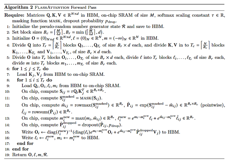 fig 12: algorithm from paper
For the above algorithm, we need the QKV matrices to be present in HBM, and assuming that the SRAM on the chip is of size M. This means that SRAM can hold M floating point numbers. We can also assume a softmax scaling constant to be \(\tau\). There is a masking function MASK and the dropout probability is there of p_drop. As you can see, we are assuming inside the attention module we are doing the calculations from equation 2 to equation 6.
 fig 13: forward pass — algorithm setup and inputs
Next we generate a pseudo random number generator R. In standard attention implementations, you could generate dropout masks once and store them. However, Flash Attention recomputes attention during the backward pass to save memory, so during forward pass we generate dropout mask using R, apply it, save R’s state. During backward pass we restore this R to the same state to regenerate the exact same dropout mask.
In the next line we set block sizes Bc = ⌈M/4d⌉, Br = min(⌈M/4d⌉, d) . This calculates the block sizes that determine how the input matrices Q, K, V are divided into smaller chunks that fit in SRAM. The d here is the head dimension of the Q, K, V matrices. Br means that its a row block and Bc means that its a column block. The division by 4d accounts for the memory needed to store 4 blocks each for the \(Q_i\), \(K_j\), \(V_j\), \(O_i\) blocks. Why min(\(\dots\), d) for Br? The min with d prevents Br from being larger than necessary. Since attention typically works with sequences, there’s no benefit to making Br > d from a computational perspective, and it might waste memory.
 fig 14: forward pass — computing block sizes
Next, we initialize O, l and m in HBM memory so that we can populate the values once the computation is done. Next, we divide Q into Tr = \(\lceil N/Br\rceil\) blocks of size Br \(\times\) d each, and divide K, V into Tc = \(\lceil N/Bc\rceil\) blocks of size Bc \(\times\) d each. We also divide O into Tr blocks of size Br \(\times\) d each, divide \(\ell\) into Tr of size Br each, divide m into Tr blocks of size Br each. This divides the output and statistics to match the Q blocks. Why this alignment?Because each \(Q_i\) block produces a corresponding output block \(O_i\) . Each row of \(Q_i\) needs its own statistics (\(\ell _i\) and \(m_i\) values). This allows processing one Q block at a time while updating its corresponding outputs.
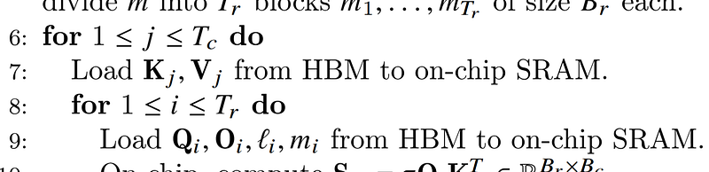 fig 15: forward pass — initialising O, \(\ell\) and m in HBM
Now we are ready and can go to the calculations. In step 7 we load \(K_j\), \(V_j\), which we have seen are blocks of key and value matrices of size Bc \(\times\) d, from HBM to on-chip SRAM. These blocks are reused across all inner loop iterations (for all \(Q_i\) blocks). This means that \(K_j\) and \(V_j\) stay in SRAM while we iterate through all Q blocks. In the inner loop, we load \(Q_i\), \(O_i\), \(\ell _i\), \(m_i\) from HBM to on-chip SRAM.
Step 10 is the unnormalized attention scores between the current Q block and K block as per equation 2. Next in step 11, is the mask function application as per equation 3. Notice that masking is a cheap operation (element-wise comparison and assignment) and thus can happen entirely on chip in SRAM.
In step 12, we compute the local statistics, \(\tilde{m}_{ij}\) which is the max score in this \(Q_i \times K_j\) block and \(\tilde{\ell}_{ij}\) which is the sum of exp(scores) in this block. Then in step 13, we update the global statistics, \(m_i\) which is the running maximum score seen so far (across all K blocks processed) and \(\ell _i\) which is the running sum of exp(scores) seen so far (properly rescaled) [see eq15 derivation above], based on the local statistics computed till now.
In step 14, we apply the dropout to the unnormalized attention weights. Notice that we are applying dropout on the unnormalised weights and not on the normalized attention which is still being computed. We’ll normalize them later when we have the final \(\ell _i\). This is fine because applying dropout before final normalization is mathematically equivalent and more efficient.
Code 5
14:    On chip, compute P_ij = dropout(P_ij, p_drop)
15:    Write O_i ← diag(ℓ_i^new)^{-1}(diag(ℓ_i)e^{m_i - m_i^new} O_i + e^{m̃_ij - m_i^new} P̃_ij^dropped V_j) to HBM.
16:    Write ℓ_i ← ℓ_i^new, m_i ← m_i^new to HBM.
17:  end for
Step 15 is the crux of the whole algorithm and the raison d’être. Here we are computing \(O_i\) based on the equation 25 which was derived earlier and writing it to HBM. Finally in step 16 we update \(\ell _i\) and \(m_i\).
Code#
Code 6
@triton.jit
def _flash_fwd_inner(
    acc, l_i, m_i, q,
    K_ptr, V_ptr,
    stride_n, stride_d,
    start_m, qk_scale,
    BLOCK_M:  tl.constexpr,
    HEAD_DIM: tl.constexpr,
    BLOCK_N:  tl.constexpr,
    STAGE:    tl.constexpr,  # 1 = non-causal full pass, 2 = causal diagonal
    offs_m:   tl.constexpr,
    offs_n:   tl.constexpr,
    N_CTX:    tl.constexpr,
):
    # — set loop bounds for this stage ————————————————————————————————
    if STAGE == 1:
        lo, hi = 0, N_CTX
    else:
        lo = start_m * BLOCK_M
        hi = (start_m + 1) * BLOCK_M
        lo = tl.multiple_of(lo, BLOCK_M)

    # — inner j-loop ——————————————————————————————————————————————————
    for start_n in range(lo, hi, BLOCK_N):
        start_n = tl.multiple_of(start_n, BLOCK_N)
        col_idx = start_n + offs_n

        # load K_j  [BLOCK_N, HEAD_DIM]
        k = tl.load(
            K_ptr + col_idx[:, None] * stride_n + tl.arange(0, HEAD_DIM)[None, :] * stride_d,
            mask=col_idx[:, None] < N_CTX, other=0.0,
        )

        # S_ij = Q_i @ K_j^T
        qk = tl.dot(q, tl.trans(k))

        if STAGE == 2:
            # causal diagonal: mask upper-triangle positions
            mask  = offs_m[:, None] >= (start_n + offs_n[None, :])
            qk    = qk * qk_scale + tl.where(mask, 0.0, -1.0e6)
            m_ij  = tl.maximum(m_i, tl.max(qk, 1))
            qk   -= m_ij[:, None]
        else:
            # exp2 trick: qk_scale = sm_scale / ln(2)
            # tl.math.exp2(qk * qk_scale) == exp(qk * sm_scale)  — exact, cheaper
            m_ij  = tl.maximum(m_i, tl.max(qk, 1) * qk_scale)
            qk    = qk * qk_scale - m_ij[:, None]

        # [Alg2 step 12]  unnormalised weights via exp2
        Pij  = tl.math.exp2(qk)        # [BLOCK_M, BLOCK_N]
        l_ij = tl.sum(Pij, 1)          # [BLOCK_M]

        # [Alg2 step 13]  correction factor and accumulator update
        alpha = tl.math.exp2(m_i - m_ij)
        acc   = acc * alpha[:, None]

        # load V_j and accumulate
        v = tl.load(
            V_ptr + col_idx[:, None] * stride_n + tl.arange(0, HEAD_DIM)[None, :] * stride_d,
            mask=col_idx[:, None] < N_CTX, other=0.0,
        )
        acc = tl.dot(Pij.to(tl.float16), v, acc)  # fp16 Pij x fp16 V -> fp32 acc
        l_i = l_i * alpha + l_ij
        m_i = m_ij

    return acc, l_i, m_i
Code 6: _flash_fwd_inner — the online-softmax inner loop
Based on the triton lang implementation for flash attention and to make it compatible to run on the free tier for google colab, we can write the flash attention implementation for Tesla T4 (Turing, sm_75, 48 KB shared memory) as shown in Code 6 and Code 7. You can go run the code in this colab link.
In Code 6 above, we have the function _flash_fwd_inner which runs inside _flash_fwd_kernel (Code 7) and implements lines 10–13 of Algorithm 2 for one column-block at a time. The STAGE constexpr selects loop bounds at compile time — STAGE=1 visits all column blocks (non-causal), STAGE=2 visits only the diagonal block where the triangular mask is actually needed. This avoids applying the expensive tl.where mask on every block when only one block needs it.
In each iteration we load \(K_j\). This computes qk = Q_i @ K_j^T, then applies the exp2 trick from the tutorial. Since qk_scale = sm_scale / ln(2) was pre-folded in the outer kernel, tl.math.exp2(qk * qk_scale) is numerically identical to exp(qk * sm_scale) but maps to a single cheaper hardware instruction. The online softmax update from Algorithm 2 line 13 then follows directly wherealpha = exp2(m_i - m_ij) rescales the old accumulator before adding the new block's contribution. V is loaded after P is computed rather than before to let the compiler reuse registers. The function returns updated acc, l_i, m_ithus avoiding HBM writes inside this inner 3function.
Code 7
@triton.jit
def _flash_fwd_kernel(
    Q_ptr, K_ptr, V_ptr,
    O_ptr, M_ptr,
    stride_z, stride_h,
    stride_n, stride_d,
    Z, H,
    N_CTX:    tl.constexpr,
    HEAD_DIM: tl.constexpr,
    BLOCK_M:  tl.constexpr,
    BLOCK_N:  tl.constexpr,
    CAUSAL:   tl.constexpr,
):
    start_m = tl.program_id(0)
    off_hz  = tl.program_id(1)

    adj     = (off_hz // H) * stride_z + (off_hz % H) * stride_h
    Q_ptr += adj
    K_ptr += adj
    V_ptr += adj
    O_ptr += adj

    offs_m = start_m * BLOCK_M + tl.arange(0, BLOCK_M)
    offs_n = tl.arange(0, BLOCK_N)

    acc = tl.zeros([BLOCK_M, HEAD_DIM], dtype=tl.float32)
    l_i = tl.zeros([BLOCK_M], dtype=tl.float32) + 1.0    # init=1 avoids div/0
    m_i = tl.zeros([BLOCK_M], dtype=tl.float32) - float("inf")

    # exp2 trick: pre-fold 1/ln(2) into the scale
    sm_scale = HEAD_DIM ** -0.5
    qk_scale = sm_scale * 1.44269504    # 1/ln(2)

    q = tl.load(
        Q_ptr + offs_m[:, None] * stride_n + tl.arange(0, HEAD_DIM)[None, :] * stride_d,
        mask=offs_m[:, None] < N_CTX, other=0.0,
    )

    if CAUSAL:
        acc, l_i, m_i = _flash_fwd_inner(
            acc, l_i, m_i, q, K_ptr, V_ptr, stride_n, stride_d,
            start_m, qk_scale, BLOCK_M, HEAD_DIM, BLOCK_N, 2, offs_m, offs_n, N_CTX,
        )
    else:
        acc, l_i, m_i = _flash_fwd_inner(
            acc, l_i, m_i, q, K_ptr, V_ptr, stride_n, stride_d,
            start_m, qk_scale, BLOCK_M, HEAD_DIM, BLOCK_N, 1, offs_m, offs_n, N_CTX,
        )

    # epilogue: merge running max + log-sum into combined log-sum-exp for backward
    m_i += tl.math.log2(l_i)
    acc  = acc / l_i[:, None]

    tl.store(M_ptr + off_hz * N_CTX + offs_m, m_i, mask=offs_m < N_CTX)
    tl.store(
        O_ptr + offs_m[:, None] * stride_n + tl.arange(0, HEAD_DIM)[None, :] * stride_d,
        acc.to(tl.float16),
        mask=offs_m[:, None] < N_CTX,
    )
Code 7: _flash_fwd_kernel — the forward-pass kernel
The _flash_fwd_kernel is the main kernel call. Here we take the four individual strides of the original [B, H, N, d] tensor. Then pointer arithmetic is used to reach this program instance’s (batch, head) slice:
Code 8
adj    = (off_hz // H) * stride_z + (off_hz % H) * stride_h
Q_ptr += adj;  K_ptr += adj;  V_ptr += adj;  O_ptr += adj
The off_hz = tl.program_id(1) encodes the flattened (batch \(\times\) head) index, and dividing/modding by H recovers the batch and head indices separately to apply their respective strides. Then the accumulators acc, l_i and m_i are initialised.
Next l_i = 1.0 rather than 0.0 is the tutorial's fix for a subtle bug: on the first iteration m_i = -inf so alpha = exp2(-inf - m_ij) = 0, meaning the old acc contribution is zeroed out correctly. But if l_i = 0 and the first block happens to be entirely masked (all -inf scores), then Pij is all zeros, l_ij = 0, and l_i stays zero — causing acc / l_i to produce NaN. Starting at 1.0 provides a safe denominator.
The after loading Q, the _flash_fwd_inner is called — once for non-causal (STAGE=1, full range), or once for the diagonal block (STAGE=2) for causal. A complete causal implementation would also call with STAGE=1 restricted to hi = start_m * BLOCK_M for the off-diagonal blocks, but this simplified version only handles the diagonal.
Finally we update m_i and acc. The first line computes log2(sum_j exp2(s_j)) — the standard log-sum-exp — by combining the running max and log of the normaliser into a single scalar per row. This is what gets stored in the M buffer and is needed for the backward pass to recompute softmax probabilities without storing the full attention matrix. The second line applies the final normalisation. The output is cast from fp32 to fp16 only at the tl.store call — all internal arithmetic stayed in fp32 throughout.
You can compare this kernel with the flash attention original kernel as shown in the flash attention repo. There its a single function call. Although that specific kernel is not used right now due to the improvements since the original paper, still there are many insights we can get from this code.
Flash Attention Backward Pass#
Since we are not saving the intermediate outputs, we need to do the backward. In this section we will derive the formulas related to efficient backward pass calculation. Then we will showcase the naive algorithm and finally go through the efficient algorithm as described in the flash attention paper.
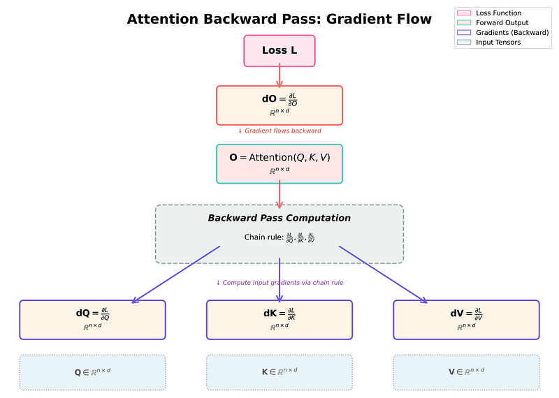 fig 16: Backward Pass though attention. Image by author
Suppose there is a scalar loss function \(L\) and because we are working in a deep learning framework such as pytorch we will be having the output gradient dO = \(\partial L/\partial O\) \(\in\) \(\mathbb{R}^{n \times d}\). From this we want to compute the input gradients dQ, dK, dV \(\in\) \(\mathbb{R}^{n \times d}\), where dQ = \(\partial L/\partial Q\), dK = \(\partial L/\partial K\) and dV = \(\partial L/\partial V\).
In the paper the derivation is there but a lot of the steps are skipped. In Linear Algebra it is important to make sure that we are differentiating in the right manner. Hence taking inspiration from Li Yuan’s blog, lets take a 3x3 matrix example to make sure our expressions are correct.
Lets assume that Q, K, V are all \(3\times 3\) matrices. So from equation 2–6, P = softmax(\(QK^T\)) is \(3\times 3\). So O = PV is \(3\times 3\). Hence dO is the gradient w.r.t. O (also \(3\times 3\)). In equations 26–28, I am showing the individual elements in P, V and O.
From equation 4–6 we can say O=PV (ignoring the dropout part for now). The next line is the expansion for a 3x3 matrix multiplication. Each element is the multiplication of the corresponding elements from rows of P and columns of V; this is shown by the subscripts. Thus, we see what each element in the O matrix means in terms of the elements of P and V in equation 29.
Now lets focus on finding dV first. Remember, V is a \(3\times 3\) matrix and \(L\) is a single scalar loss number. So when we write \(\partial L/\partial V\), we’re asking: “how does the loss change with respect to each individual element of V?” Since V has 9 elements, we get 9 partial derivatives. In equation 30 above the matrix just organizes them in the same positions as their corresponding elements in V.
Lets focus on finding dV element by element. We start with \(\partial L/\partial v11\). Now \(L\) doesn’t depend on \(v_{11}\) directly. It depends on \(v_{11}\) only through O as shown in fig 16 above. So, using the multivariate chain rule, to find how \(L\) changes when \(v_{11}\) changes, we need to account for every “path” through which \(v_{11}\) affects L. This concept is explained in this stackexchange link.
Observe that in the expansion of O in equation 29, there are 3 elements that contain v11: o11, o21, o31. And from equation 29, we expand these values above in eq 31–33.
Next in eq 34–36, we are taking the derivative of o11, o21 and o31 and from equation 31–33 they are p11, p21 and p31.
So as per the multivariate chain rule as discussed, we can combine all the partial derivatives in eq 37. And then, in eq 38, replace the values of \(\partial O_{11}/\partial v_{11}\), \(\partial O_{21}/\partial v_{11}\) and \(\partial O_{31}/\partial v_{11}\) using equation 34–36. In the next line in eq 39, we are just replacing with notation, \(\partial L/\partial v\) as dv and \(\partial L/\partial o\) as do as per definition.
Using the same logic as we have done for \(dv_{11}\), as shown in equation 39, expand for the other elements in the matrix for dV in equation 30 from \(dv_{12}\) to \(dv_{33}\). Try it out on your own and see if it matches with the ones shown in equation 40–47.
In equation 48, we are replacing these expansions from equation 39–47 in the respective places in the matrix for dV in equation 30. Observe that this becomes like a matrix multiplication form and hence we can break into two matrices, one for P and one for O inequation 49. Thus in equation 50, we can write in the matrix notation for dV in terms of P and dO.
The gradients of dQ and dK are slightly more complicated so we need to go through the gradients of dP and dS first.
Now you should be able to derive for dP using same multivariate chain rule as we have done for finding dV. Once you have done this come back and see the derivation above in equation 51.
Now lets go over the derivation of dS as well.
Equation 52 is the definition of P in terms of S as per equation 4. Next in equation 53, we can expand this in matrix terms where each term is the exp of the corresponding value in S and the denominator is the sum of the exp in the corresponding rows.
This means that applying the same multivariate chain rule while deriving dV, for dS, we can say that the first value \(\partial L/\partial s_{11}\) is the sum of the partials going through \(p_{11}\), \(p_{12}\) and \(p_{13}\) since these are the values which have the terms \(s_{11}\). This is shown above in equation 54.
So, to resolve equation 54 and find \(\partial L/\partial s_{11}\), we need to find \(\partial p_{11}/\partial s_{11}\), \(\partial p_{12}/\partial s_{11}\) and \(\partial p13/\partial s_{11}\), which we don't know here. \(\partial L/\partial p_{11}\) and the corresponding values are right now known because dP is known from equation 51. Lets go through them one by one.
First, we take the value of \(p_{11}\) from equation 53. If we take the derivative and apply the quotient rule as shown here, we can do some algebraic manipulations and arrive at equation 56, where \(\partial p_{11}/\partial s_{11}\) = \(p_{11}\) — \(p^2_{11}\).
Using the same logic, from eq 53 in matrix form we can take out the value of \(p_{12}\) as shown in eq 57. The for the partial derivative we can apply the quotient rule as shown in eq 58. The denominator is a square, which means product of two sums of exponentials and in the numerator also there is a product of two exponentials. So we can write the overall expression as the product of two fractions which resolve to product of \(p_{11}\) and \(p_{12}\).
Similarly we can derive for \(\partial p_{13}/\partial s_{11}\) which is the negative product of \(p_{11}\) and \(p_{13}\). Make sure that you understand the steps between 55–59 and derive this yourself.
Now we can take eq 54 and replace the corresponding \(\partial p/\partial s\) partials that we have derived in eq 56, 59 and 60 and replace them here. Thus we arrive at equation 61.
Similarly find the expressions for the partial derivative \(s_{12}\) to \(s_{33}\). I have not written the derivation here, but you should be able to do this yourself now. Follow the same steps from eq 52 to 61.
Above eq 70 is if we write all these expressions that we have derived from eq 61 to 69 in matrix form.
Now we are not able to do things as neatly as when we were deriving for dV. For resolving dS, lets do things in a row wise fashion. The matrix in equation 70 can be thought of as a column vector of three vectors as shown in equation 71.
Equation 72 is just taking the first value in the column vector of equation 79 and showing it in expanded form as in equation 70.
Now I can decompose the vector in equation 72 into product of a vector of \(\partial L/\partial p\) ‘s and a matrix where the values are the p terms.
Next, we can take the vector [\(\partial L/\partial p_{11}\) \(\partial L/\partial p_{12}\) \(\partial L/\partial p_{13}\)] and write it as \(\partial L/\partial P_1\) showing that it's the 1st row in the \(\partial L/\partial P\) matrix. This is in accordance with the left side of the equals sign \(\partial L/\partial S_1\) which also means that this is the 1st row in the \(\partial L/\partial S\) matrix. This formulation will soon help us, you will see.
We also take the p term matrix and separate it into the single terms matrix and the product terms matrix. Since only the diagonal elements in eq 73 have single terms hence in the single term matrices apart from the diagonals all others are 0. Notice that all the product terms have a negative (-) sign with them, so we can take it out. So this becomes a difference of two matrices.
Next, we can remove the brackets and propagate the \(\partial L/\partial P_1\) as shown in eq 75.
Next in eq 76, in the first term we change \(\partial L/\partial P\) to [\(\partial L/\partial p_{11}\) \(\partial L/\partial p_{12}\) \(\partial L/\partial p_{13}\)] as we intend to do the multiplication after this. For the second term, notice that we can decompose the matrix in eq 75 to this multiplication of a column vector and a row vector.
Next in eq 77, we multiply the row vector and matrix in the 1st term, which results in the row vector with \(\partial L/\partial p_x\) \(p_x\). The second term we can write as the product \(P_1^T P_1\).
Next in eq 78 and then in eq 79, we can take the 1st term in the expression and convert it into element wise multiplication of the two row vectors \(\partial L/\partial P_1\) and \(P_1\).
In equation 51 we have dP = dOV. So we can write it in row vector form above. This we can replace for \(\partial L/\partial P_1\) in equation 79 and we get eq 80.
From eq 80, you can take the \(V^T P^T\) part and from the rules in linear algebra you can write it as \((PV)^T\).
As per definition O=PV and if you analyse equation 29, then converting this into row wise, \(O_1=P_1V\). This we can replace in eq 81 to arrive at eq 82. Now all the terms of the expression is in terms of the 1st row vector. Taking cue from this expression, we can write the full matrix form.
Now, let's define the term D for the full row which would stand for \(dO_1\bigodot O_1^T\). This is the same as doing a row sum for the element wise multiplication or Hadamard product for the values in the row of \(dO_1\) and \(O_1\). This is a dot product of two d-dimensional vectors and is a scalar. This is shown in eq 83.
If we insert for \(D_1\) in eq 82, this means that we can write the whole equation as element wise operation as shown in eq 84. And we can take \(P_1\) out which would convert this to one subtraction and one multiplication.
Eq 85 means that for a specific value in dS matrix is dependent on having D value for the full row. This is shown in eq 86. If you are sad that we are not able to do a full steaming like we did in forward pass for softmax, atleast there is the consolation prize that \(D_1\) is a scalar. If you can think about how to optimise this part as well and if you are able to achieve this that would be a big milestone.
Now that we know dS, we can attempt at dQ and dK. Lets go through the derivations below.
Above we can see \(S=Q\cdot K^T\), this we can expand in matrix form. This helps us to formulate \(\partial L/\partial q_{11}\) as per the multivariate chain rule. Replacing the corresponding values for \(\partial s_{xx}/\partial q_{xx}\) from the corresponding values in the matrix form, we arrive at equation 87.
Till now we have done this a lot of times, so try out the derivations for \(\partial L/\partial q_{12}\) to \(\partial L/\partial q_{33}\). Check your answer with equations 88–95 above.
Thus we can compile eq 87–95 in matrix form. This gives such \(dQ=dS\cdot K\) as shown in eq 96. Observe that we have the values of dS in eq 86.
Similarly, we can derive for \(dK=dS^T\cdot Q\) as shown above in eq 97. I have jumped a lot of steps, so verify this yourself as an exercise and make sure you understand the derivations.
Compiling all the derivations that we have done below in eq 98.
Now for the backward pass algorithm based on the equations we have derived could look like this.
- Compute dV, save to HBM
- Compute dP, save to HBM.
- Compute dS, save to HBM.
- Finally compute dQ and dK, probably together as they depend on dS and save to HBM.
Instead of computing the backward pass like above, the authors of the flash attention paper were able to find a tiled approach to the backward pass as shown below.
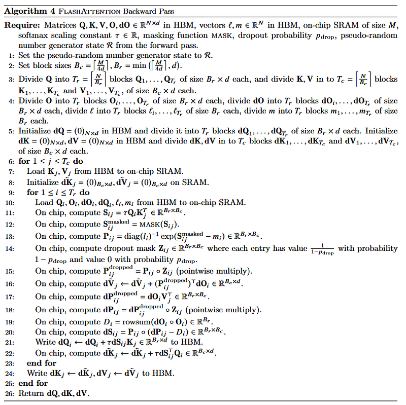 fig 17: backward pass in the flash attention paper arxiv.org/pdf/2205.14135
Similar to the discussion on the forward pass earlier, lets go through this line by line.
 fig 18: backward pass — overview
Lets start with the requirements, as we have discussed in the start of the derivations for the backward pass between eq 26–29, for the backward pass we need Q, K, V, O and dO present in HBM memory. We will need the vectors \(\ell\), m \(\in\) \(\mathbb{R}^N\) which are the logsumexp and max values from the forward pass, stored in HBM. We will need the hyper parameters in SRAM — \(\tau\) \(\in\) \(\mathbb{R}\) which is the softmax scaling constant, p_drop— Dropout probability and MASK — Masking function (e.g., for causal attention), as defined in the forward pass. For the state of the algorithm, we need \(\mathcal{R}\) — Pseudo-random number generator state. This must be the same as forward pass to reproduce dropout mask.
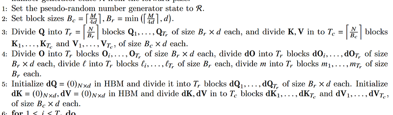 fig 19: backward pass — requirements
Now steps 1–5 is about setup. In step 1, we initialise the RNG to the same state as used in the forward pass. This is important because we want to reproduce the exact dropout mask that was applied during the forward pass. This ensures that the gradient computation is consistent with the elements that were actually dropped.
In step 2, we set the column block size B꜀ and row block size \(B_r\). As seen in the forward pass, the factor of 4 is to accout for all the intermediate matrices in SRAM simultaneously. Using this in steps 3 and 4, we partition Q, K, V into T꜀ = \(\lceil N/B\)꜀\(\rceil\). Thus T꜀ is the number of column blocks to cover all N tokens. Similarly we divide O, dO, \(\ell\) and m into \(T_r=\lceil N/B_r\rceil\) blocks where \(T_r\) is the number of row blocks.
Similar to the inputs, we setup the outputs in step 5. We 0-initialise dQ in \(T_r\) blocks and K, V in T꜀ blocks so that they match K, V’s column wise processing. This is done so that we can accumulate results as we go.
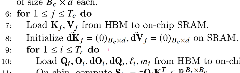 fig 20: backward pass — setup and outputs
Similar to how we had seen in the forward pass, there is this overall nested loop structure: for 1 \(\le\) j \(\le\) T꜀ do # Outer loop \(\dots\) for 1 \(\le\) i \(\le\) \(T_r\) do # Inner loop. This creates a double loop that processes \(T_r\) \(\times\) T꜀ block pairs, where the outer loop (j) iterates over K, V blocks (column wise chunks) and the inner loop (i) iterates over Q, O, dO blocks (row wise chunks). Thus, with each i, j pair, we compute attention over \(Q_i\) and \(K_j/V_j\).
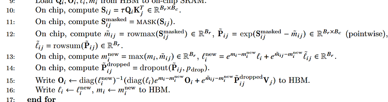 fig 21: forward pass benchmark
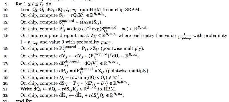 fig 22: backward pass benchmark
If you compare the forward pass with the backward pass, many of the operations are the same. Computing attention scores \(S=QK^T\) is the same in step 11 in backward with step 10 in forward. Then the mask is calculated which is the same in step 12 in backward and step 11 in forward. Then next the same dropout is applied to both attention probabilities. The only difference is that in case of backward the dropout mask Z needs to be the same that is applied in forward and then pointwise multiplication is done. So still step 15 in backward the steps are mostly similar to the forward process because the same tensors are recomputed. That is why I have added a screenshot for the forward process as well.
Since this is the backward process, we have to compute dV, dP, dS, dQ, dK as per equation 95. This is done between steps 16 and 22.
In step 16, we are computing dV as per equation 95: \(dV = P^T dO\). Hence since this is a tiled algorithm, we are accumulating \(dV_j\) contributions from all query blocks i.
Again as per eq 95 for dP, we implement the algorithm for computing dP. Since the chain for the gradients is like loss \(\to\) dO \(\to\) dP(dropped) \(\to\) dP \(\to\) dS \(\to\) dQ, dK, hence the calculation is for dP(dropped) in step 17. After that we need to apply the dropout Z to arrive at the actual dP.
Moving in step 19, on based on equation 86, we need to calculate \(D_i\), so we calculate \(D_i\) = rowsum(\(dO\odot O\)) for the row as defined in eq 83. Notice that although we are loading one full row of O, still this can be done element by element in a vectorised form.
Now that we have \(D_i\), we can calculate \(dS_{ij}\) as per eq 86. Notice that dS is calculated element by element here and agrees with eq 86.
Now that we have dS for a specific row and column, we can implement eq 96 and 97 and accumulate for dQ and dK.
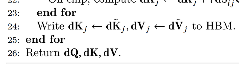 fig 23: backward pass — dQ accumulation step
We have implemented all the expressions that we had derived for the backward pass. So we write dK and dV for the specific column to HBM and once all loops are done we return the three gradient matrices.
Code#
Now lets go through the code for the backward process
Attention backward preprocessing part
Code 9
@triton.jit
def _attn_bwd_preprocess(
    O_ptr, DO_ptr,          # [B*H, N, d]
    Delta_ptr,              # [B*H, N]  output
    Z, H, N_CTX,
    BLOCK_M: tl.constexpr,
    HEAD_DIM: tl.constexpr,
):
    off_m = tl.program_id(0) * BLOCK_M + tl.arange(0, BLOCK_M)
    off_hz = tl.program_id(1)
    off_d = tl.arange(0, HEAD_DIM)

    o  = tl.load(O_ptr  + off_hz * HEAD_DIM * N_CTX + off_m[:, None] * HEAD_DIM + off_d[None, :])
    do = tl.load(DO_ptr + off_hz * HEAD_DIM * N_CTX + off_m[:, None] * HEAD_DIM + off_d[None,
:]).to(tl.float32)

    # delta = rowsum(o * do)  [BLOCK_M]
    delta = tl.sum(o * do, axis=1)
    tl.store(Delta_ptr + off_hz * N_CTX + off_m, delta)
Code 9: _attn_bwd_preprocess — precompute the D vector
The preprocessing kernel in Code 9 above computes the D buffer. During the backward pass calculation, the calculation of dS is dependent on D_i = rowsum(O_i ⊙ dO_i) for every query row i (check eq 98, 83 and algo 4 step 19, 20). Since the dependency is only on O and dO and not on K and V, we can compute it once upfront and store it in the HBM as a reusable [B·H, N] buffer. The alternative would be to recompute it inside every iteration of the hot dK/dV inner loop, wasting compute and register pressure.
In the forward pass, the loop structure is straightforward: for each Q row-block i, stream over all K/V column-blocks j. Each program instance owns one i and accumulates its output O_i completely before writing to HBM. But things are different in the backward pass. There is a difference in the dependency structure.
Code 10
dV_j  = Σ_i  P_ij^T dO_i          — sums over ALL query rows i, for fixed j
dK_j  = Σ_i  τ · dS_ij^T Q_i      — sums over ALL query rows i, for fixed j
dQ_i  = Σ_j  τ · dS_ij K_j        — sums over ALL key cols  j, for fixed i
We can try to write all the operations on a single go essentially opting for a fused kernel. In that case we are writing for each (i, j) block computing all three gradients simultaneously. We would be writing partial dK/dV buffers and reducing afterwards. Thus the overall memory that would be required would blow up. As a solution two separate kernels are written, _attn_bwd_dkdv and _attn_bwd_dq. One would do dV, dK together and another would work on dQ.
Attention backward function for dk dv
Code 11
@triton.jit
def _attn_bwd_dkdv(
    dk, dv,
    Q_ptr, k, v, sm_scale,
    DO_ptr,
    M_ptr, D_ptr,
    stride_tok, stride_d,
    H, N_CTX,
    BLOCK_M1:  tl.constexpr,
    BLOCK_N1:  tl.constexpr,
    HEAD_DIM:  tl.constexpr,
    start_n, start_m, num_steps,
    MASK: tl.constexpr,
):
    offs_m = start_m + tl.arange(0, BLOCK_M1)
    offs_n = start_n + tl.arange(0, BLOCK_N1)
    offs_k = tl.arange(0, HEAD_DIM)

    # Transposed Q pointer: shape [HEAD_DIM, BLOCK_M1] for dot(k, qT)
    qT_ptrs  = Q_ptr  + offs_m[None, :] * stride_tok + offs_k[:, None] * stride_d
    do_ptrs  = DO_ptr + offs_m[:, None] * stride_tok + offs_k[None, :] * stride_d

    tl.static_assert(BLOCK_N1 % BLOCK_M1 == 0)
    curr_m = start_m
    for _ in range(num_steps):
        qT = tl.load(qT_ptrs)                          # [HEAD_DIM, BLOCK_M1]
        offs_m = curr_m + tl.arange(0, BLOCK_M1)
        m = tl.load(M_ptr + offs_m)                    # [BLOCK_M1] log-sum-exp

        # Recompute P_ij^T = exp2(K_j Q_i^T - M_i)   [BLOCK_N1, BLOCK_M1]
        qkT = tl.dot(k, qT)                            # [BLOCK_N1, BLOCK_M1]
        pT  = tl.math.exp2(qkT - m[None, :])

        if MASK:
            # causal: token j can only attend to token i if i >= j
            mask = (offs_m[None, :] >= offs_n[:, None])
            pT   = tl.where(mask, pT, 0.0)

        do = tl.load(do_ptrs)                          # [BLOCK_M1, HEAD_DIM]

        # dV_j += P_ij^T dO_i   [Alg4 line 16]
        dv += tl.dot(pT.to(tl.float16), do)

        # dS_ij^T = P_ij^T * (dO_i V_j^T - delta_i)  [Alg4 lines 17,19,20]
        Di   = tl.load(D_ptr + offs_m)                          # [BLOCK_M1] delta
        dpT  = tl.dot(v, tl.trans(do)).to(tl.float32) # [BLOCK_N1, BLOCK_M1]
        dsT  = pT * (dpT - Di[None, :])

        # dK_j += tau * dS_ij^T Q_i   [Alg4 line 22]
        dk  += tl.dot(dsT.to(tl.float16), tl.trans(qT))

        curr_m     += BLOCK_M1
        qT_ptrs    += BLOCK_M1 * stride_tok
        do_ptrs    += BLOCK_M1 * stride_tok

    return dk, dv
Code 11: _attn_bwd_dkdv — accumulate dK and dV for a fixed K/V block
In Code 11 above, for a fixed K/V column block j, we stream over all Q row-blocks and accumulates dK_j and dV_j . We are implementing the steps 15, 16, 17, 18, 20 and 22 from the backward pass algorithm 4 that was discussed earlier.
Code 12
qkT = tl.dot(k, qT) # [BLOCK_N1, BLOCK_M1]pT = tl.math.exp2(qkT - m[None, :])
Notice that here \(P_{ij}\) is never stored — we recompute it on on the fly from the saved log-sum-exp M . Because qT_ptrs has shape [HEAD_DIM, BLOCK_M1] in index space — dimensions are swapped relative to the usual [BLOCK_M1, HEAD_DIM] layout. Loading from this pointer pattern gives qT = [HEAD_DIM, BLOCK_M1] directly, so tl.dot(k, qT) computes K_j Q_i^T as [BLOCK_N1, HEAD_DIM] × [HEAD_DIM, BLOCK_M1] = [BLOCK_N1, BLOCK_M1] without needing an explicit tl.trans call. Thus we are able to directly arrive at pT.
Code 13
if MASK: mask = (offs_m[None, :] >= offs_n[:, None]) pT = tl.where(mask, pT, 0.0)
Because pT is transposed — rows are key-block positions j, columns are query-block positions i — we have to specify the causal condition asi >= j (query token can attend to key token only if key comes before or at query position). Zeroing masked positions in pT before accumulating into dV and dK ensures those positions contribute nothing to the gradients. This is consistent with how the causal mask was applied in the forward pass.
Code 14
Di   = tl.load(D_ptr + offs_m)                 # [BLOCK_M1] delta
dpT  = tl.dot(v, tl.trans(do)).to(tl.float32) # [BLOCK_N1, BLOCK_M1]
dsT  = pT * (dpT - Di[None, :])
dk  += tl.dot(dsT.to(tl.float16), tl.trans(qT))
For the dk calculation, we load Di is the delta vector [BLOCK_M1] precomputed by _attn_bwd_preprocess. We compute dpT and dsT as per steps 18 and 20. Then we calculate the current dk_j and accumulate into dk.
Attention backward function for dq
Code 15
@triton.jit
def _attn_bwd_dq(
    dq, q, K_ptr, V_ptr,
    do, m, D_ptr,
    stride_tok, stride_d,
    H, N_CTX,
    BLOCK_M2:  tl.constexpr,
    BLOCK_N2:  tl.constexpr,
    HEAD_DIM:  tl.constexpr,
    start_m, start_n, num_steps,
    MASK: tl.constexpr,
):
    offs_m = start_m + tl.arange(0, BLOCK_M2)
    offs_n = start_n + tl.arange(0, BLOCK_N2)
    offs_k = tl.arange(0, HEAD_DIM)

    # Transposed K and V pointers
    kT_ptrs = K_ptr + offs_n[None, :] * stride_tok + offs_k[:, None] * stride_d
    vT_ptrs = V_ptr + offs_n[None, :] * stride_tok + offs_k[:, None] * stride_d

    Di = tl.load(D_ptr + offs_m)                    # [BLOCK_M2] delta

    tl.static_assert(BLOCK_M2 % BLOCK_N2 == 0)
    curr_n = start_n
    for _ in range(num_steps):
        kT = tl.load(kT_ptrs)                       # [HEAD_DIM, BLOCK_N2]
        vT = tl.load(vT_ptrs)                       # [HEAD_DIM, BLOCK_N2]

        # Recompute P_ij = exp2(Q_i K_j^T - M_i)   [BLOCK_M2, BLOCK_N2]
        qk = tl.dot(q, kT)                          # note: kT already pre-scaled
        p  = tl.math.exp2(qk - m)

        if MASK:
            offs_n = curr_n + tl.arange(0, BLOCK_N2)
            mask   = (offs_m[:, None] >= offs_n[None, :])
            p      = tl.where(mask, p, 0.0)

        # dS_ij = P_ij * (dO_i V_j^T - delta_i)
        dp = tl.dot(do, vT).to(tl.float32)          # [BLOCK_M2, BLOCK_N2]
        ds = p * (dp - Di[:, None])

        # dQ_i += tau * dS_ij K_j  (K was pre-multiplied by tau*RCP_LN2 in Python)
        dq += tl.dot(ds.to(tl.float16), tl.trans(kT))

        curr_n  += BLOCK_N2
        kT_ptrs += BLOCK_N2 * stride_tok
        vT_ptrs += BLOCK_N2 * stride_tok

    return dq
Code 15: _attn_bwd_dq — accumulate dQ for a fixed query block
The function _attn_bwd_dq in Code 15 above is the mirror image of _attn_bwd_dkdv. Before we fixed j and streamed over query rows, now we are fixing i and streaming over the K/V column blocks. In this function, we are implementing step 21 from the algorithm dQ_i += τ · dS_ij K_j.
Another difference is in the calculation of Di. In that function, _attn_bwd_dkdv ,Di was loaded inside the loop because offs_m changed each iteration as the function stepped through different Q row-blocks. Here offs_m is fixed for the entire function call — this is the row-block we own — so Di is loaded once before the loop and reused across all num_steps iterations. Thus we are savingnum_steps HBM loads compared to _attn_bwd_dkdv.
Also for the masking, we need to have query row index >= key column index. Thus the condition offs_m[:, None] >= offs_n[None, :]is the standard causal mask in the natural (non-transposed) orientation. The other calculations, such as the recomputation of \(P_ij\), the delta subtraction, the mask application, are mostly identical to _attn_bwd_dkdv.
The outer function for attention backward
Code 16
@triton.jit
def _attn_bwd(
    Q_ptr, K_ptr, V_ptr, sm_scale,
    DO_ptr,
    DQ_ptr, DK_ptr, DV_ptr,
    M_ptr, D_ptr,
    stride_z, stride_h, stride_tok, stride_d,
    H, N_CTX,
    BLOCK_M1:        tl.constexpr,
    BLOCK_N1:        tl.constexpr,
    BLOCK_M2:        tl.constexpr,
    BLOCK_N2:        tl.constexpr,
    BLK_SLICE_FACTOR: tl.constexpr,
    HEAD_DIM:        tl.constexpr,
    CAUSAL:          tl.constexpr,
):
    LN2: tl.constexpr = 0.6931471824645996  # ln(2) - used to rescale dQ

    bhid     = tl.program_id(2)
    off_chz  = (bhid * N_CTX).to(tl.int64)
    adj      = (stride_h * (bhid % H) + stride_z * (bhid // H)).to(tl.int64)
    pid      = tl.program_id(0)

    # Offset all pointers to this (batch, head)
    Q_ptr  += adj;  K_ptr  += adj;  V_ptr  += adj
    DO_ptr += adj;  DQ_ptr += adj;  DK_ptr += adj;  DV_ptr += adj
    M_ptr  += off_chz;  D_ptr  += off_chz

    offs_k  = tl.arange(0, HEAD_DIM)
    start_n = pid * BLOCK_N1
    offs_n  = start_n + tl.arange(0, BLOCK_N1)

    # Load K_j, V_j - stay in SRAM throughout dK/dV loop
    k = tl.load(K_ptr + offs_n[:, None] * stride_tok + offs_k[None, :] * stride_d)
    v = tl.load(V_ptr + offs_n[:, None] * stride_tok + offs_k[None, :] * stride_d)

    dv = tl.zeros([BLOCK_N1, HEAD_DIM], dtype=tl.float32)
    dk = tl.zeros([BLOCK_N1, HEAD_DIM], dtype=tl.float32)

    MASK_BLOCK_M1: tl.constexpr = BLOCK_M1 // BLK_SLICE_FACTOR

    if CAUSAL:
        # Diagonal block: Q rows that overlap with this K/V column - needs mask
        start_m  = start_n
        num_steps = BLOCK_N1 // MASK_BLOCK_M1
        dk, dv = _attn_bwd_dkdv(
            dk, dv, Q_ptr, k, v, sm_scale, DO_ptr, M_ptr, D_ptr,
            stride_tok, stride_d, H, N_CTX,
            MASK_BLOCK_M1, BLOCK_N1, HEAD_DIM,
            start_n, start_m, num_steps, MASK=True,
        )
        start_m += num_steps * MASK_BLOCK_M1
    else:
        start_m = 0

    # Non-masked Q row-blocks (all rows above the diagonal, or all rows if non-causal)
    num_steps = (N_CTX - start_m) // BLOCK_M1
    dk, dv = _attn_bwd_dkdv(
        dk, dv, Q_ptr, k, v, sm_scale, DO_ptr, M_ptr, D_ptr,
        stride_tok, stride_d, H, N_CTX,
        BLOCK_M1, BLOCK_N1, HEAD_DIM,
        start_n, start_m, num_steps, MASK=False,
    )

    # Write dV and dK (dK is scaled by sm_scale - applied once here, not per block)
    dv_ptrs = DV_ptr + offs_n[:, None] * stride_tok + offs_k[None, :] * stride_d
    tl.store(dv_ptrs, dv)
    dk *= sm_scale
    dk_ptrs = DK_ptr + offs_n[:, None] * stride_tok + offs_k[None, :] * stride_d
    tl.store(dk_ptrs, dk)

    # --- dQ section -----------------------------------------------------------
    # The same program instance also computes dQ for one Q row-block.
    # This amortises the kernel launch overhead and keeps Q-side work local.
    start_m = pid * BLOCK_M2
    start_n = 0
    offs_m  = start_m + tl.arange(0, BLOCK_M2)

    q  = tl.load(Q_ptr  + offs_m[:, None] * stride_tok + offs_k[None, :] * stride_d)
    dq = tl.zeros([BLOCK_M2, HEAD_DIM], dtype=tl.float32)
    do = tl.load(DO_ptr + offs_m[:, None] * stride_tok + offs_k[None, :] * stride_d)
    m  = tl.load(M_ptr  + offs_m[:, None])  # [BLOCK_M2, 1] log-sum-exp

    MASK_BLOCK_N2: tl.constexpr = BLOCK_N2 // BLK_SLICE_FACTOR

    if CAUSAL:
        # Diagonal block for dQ
        end_n     = start_m + BLOCK_M2
        num_steps = BLOCK_M2 // MASK_BLOCK_N2
        dq = _attn_bwd_dq(
            dq, q, K_ptr, V_ptr, do, m, D_ptr,
            stride_tok, stride_d, H, N_CTX,
            BLOCK_M2, MASK_BLOCK_N2, HEAD_DIM,
            start_m, end_n - num_steps * MASK_BLOCK_N2, num_steps, MASK=True,
        )
        end_n    -= num_steps * MASK_BLOCK_N2
        num_steps = end_n // BLOCK_N2
        start_n   = end_n - num_steps * BLOCK_N2
    else:
        num_steps = N_CTX // BLOCK_N2

    dq = _attn_bwd_dq(
        dq, q, K_ptr, V_ptr, do, m, D_ptr,
        stride_tok, stride_d, H, N_CTX,
        BLOCK_M2, BLOCK_N2, HEAD_DIM,
        start_m, start_n, num_steps, MASK=False,
    )

    # dQ was accumulated with K pre-scaled by sm_scale*RCP_LN2 in Python.
    # Multiply by LN2 to cancel the RCP_LN2 factor, recovering true dQ.
    dq *= LN2
    dq_ptrs = DQ_ptr + offs_m[:, None] * stride_tok + offs_k[None, :] * stride_d
    tl.store(dq_ptrs, dq)
Code 16: _attn_bwd — the outer backward kernel that orchestrates the others
Finally we have the outer function _attn_bwd (Code 16) which is the only kernel that PyTorch's autograd actually launches. It orchestrates the entire backward pass by calling _attn_bwd_preprocess, _attn_bwd_dkdv and _attn_bwd_dq internally.
Code 17
bhid    = tl.program_id(2)
off_chz = (bhid * N_CTX).to(tl.int64)
adj     = (stride_h * (bhid % H) + stride_z * (bhid // H)).to(tl.int64)
pid     = tl.program_id(0)
Q_ptr  += adj;  K_ptr  += adj;  V_ptr  += adj
DO_ptr += adj;  DQ_ptr += adj;  DK_ptr += adj;  DV_ptr += adj
M_ptr  += off_chz;  D_ptr  += off_chz
Here in axis 2, we index the flattened (batch, head) pair and index 0 is to identify which K/V column-block this instance owns. So the total number of program instances is (N/BLOCK_N1) × B×H, meaning every K/V column-block for every (batch, head) pair runs in parallel. Because dK and dV are indexed by j, the choice is to index by j (K/V column block) rather than i (Q row block). This gives each instance exclusive ownership of one j avoids any write conflicts when accumulating those gradients. K and V for a particular column block are loaded once and stay in SRAM for the entire dK/dV section. We initialisedk and dv to zero and accumulate contributions from every Q row-block. Thus we have one [BLOCK_N1, HEAD_DIM] tile each for K and V, resident throughout, rather than reloading them for each Q row-block.
Code 18
start_n = pid * BLOCK_N1
offs_n  = start_n + tl.arange(0, BLOCK_N1)
k = tl.load(K_ptr + offs_n[:, None] * stride_tok + offs_k[None, :] * stride_d)
v = tl.load(V_ptr + offs_n[:, None] * stride_tok + offs_k[None, :] * stride_d)
dv = tl.zeros([BLOCK_N1, HEAD_DIM], dtype=tl.float32)
dk = tl.zeros([BLOCK_N1, HEAD_DIM], dtype=tl.float32)
dk, dv calculations
In the next section is the dk, dv calculations. K and V for a particular column block are loaded once and stay in SRAM for the entire dK/dV section. dk and dv are initialised to zero here and will accumulate contributions from every Q row-block.
Code 19
MASK_BLOCK_M1: tl.constexpr = BLOCK_M1 // BLK_SLICE_FACTOR   # = 32 // 2 = 16
if CAUSAL:
    start_m   = start_n
    num_steps = BLOCK_N1 // MASK_BLOCK_M1
    dk, dv = _attn_bwd_dkdv(
        ..., start_n, start_m, num_steps, MASK=True,
    )
    start_m += num_steps * MASK_BLOCK_M1
else:
    start_m = 0
In the causal attention case, column block j (at position start_n) can only receive gradient contributions from query rows i >= j. The diagonal block — where query row and key column indices overlap — needs a per-element triangular mask. That is why we call _attn_bwd_dkdv first with MASK=True for just this diagonal region, using the finer tile size MASK_BLOCK_M1 = BLOCK_M1 // BLK_SLICE_FACTOR. The finer tile is needed because within the diagonal block only half the elements on average are unmasked. The idea is using a smaller BLOCK_M1 reduces wasted computation on masked positions. After the masked call processes num_steps * MASK_BLOCK_M1 rows, start_m is advanced to the first fully unmasked row-block. From that point every entry in our column block is valid, so the unmasked call runs at full efficiency with the larger BLOCK_M1 tile. After the masked call, start_m is advanced past the diagonal so the unmasked call begins immediately below it.
Code 20
num_steps = (N_CTX - start_m) // BLOCK_M1
dk, dv = _attn_bwd_dkdv(
    ..., start_n, start_m, num_steps, MASK=False,
)
In non causal attention, we dont need to think so much. All Q row-blocks strictly below the diagonal (i.e. i > j, rows that unconditionally attended to key position j) are processed without masking. We are specifyingstart_m = 0 so this single call covers the entire sequence. For causal attention it covers everything below the diagonal.
The curious case of start_m
I want to cover the logic surrounding start_m in slightly more detail as that part is not obvious. Let us use a concrete example. Say N=8, BLOCK_N1=4, BLOCK_M1=4, MASK_BLOCK_M1=2, BLK_SLICE_FACTOR=2. This program instance owns column block j=1, so start_n = 1 * 4 = 4 meaning it handles key tokens 4,5,6,7. Consider the full \(8\times 8\) attention matrix where rows are query tokens (i) and columns are key tokens (j). Causal masking means token i can only attend to token j if j <= i:
Code 21
key cols:    0 1 2 3 | 4 5 6 7
             --------|--------
query row 0: ✓ . . . | . . . .   ← cannot attend to keys 4-7
query row 1: ✓ ✓ . . | . . . .
query row 2: ✓ ✓ ✓ . | . . . .
query row 3: ✓ ✓ ✓ ✓ | . . . .
             --------|--------
query row 4: ✓ ✓ ✓ ✓ | ✓ . . .   ← our column block starts here
query row 5: ✓ ✓ ✓ ✓ | ✓ ✓ . .
query row 6: ✓ ✓ ✓ ✓ | ✓ ✓ ✓ .
query row 7: ✓ ✓ ✓ ✓ | ✓ ✓ ✓ ✓
Notice that there are some blocks where rows are fully masked, some blocks where rows are partially masked and some blocks where rows are fully unmasked. Our column block covers key tokens 4–7 (the right half). The ✓ marks in our column block's region are:
Code 22
query row 4: ✓ . . .    ← partial row, needs mask
query row 5: ✓ ✓ . .    ← partial row, needs mask
query row 6: ✓ ✓ ✓ .    ← partial row, needs mask
query row 7: ✓ ✓ ✓ ✓    ← full row, needs mask
Rows 0–3 have zero entries in our column block. They contribute nothing to dK or dV, so we skip them entirely. Rows 4–7 all intersect our column block and need processing. But rows 4–7 are the diagonal block — the block where query row index and key column index overlap. Every single one of them needs the per-element triangular mask because some positions are valid and some are not. There are no fully unmasked rows for this particular instance. For column block j=0 (key tokens 0–3) every query row 0–7 attends to all those keys, so rows 0–7 would be unmasked.
Now let's consider a case with both masked and unmasked rows. Consider N=16, BLOCK_N1=4, BLOCK_M1=4, MASK_BLOCK_M1=2. Program instance owns column block j=1, key tokens 4–7.
Code 23
key cols:    0-3 | 4-7 | 8-11 | 12-15
             ----|-----|------|------
query rows 0-3:  |  .  |      |         ← all zero in our block, skip
query rows 4-7:  |  ▲  |      |         ← diagonal, needs mask
query rows 8-11: |  ✓  |      |         ← fully unmasked
query rows12-15: |  ✓  |      |         ← fully unmasked
▲ = partial (diagonal block), ✓ = full (all entries valid).
Code 24
if CAUSAL:
    start_m   = start_n          # = 4  (skip rows 0-3, start at diagonal)
    num_steps = BLOCK_N1 // MASK_BLOCK_M1   # = 4 // 2 = 2 steps of size 2
    dk, dv = _attn_bwd_dkdv(..., start_n=4, start_m=4, num_steps=2, MASK=True)
    # this processes query rows 4-5 (step 1) and 6-7 (step 2) with mask
    start_m += num_steps * MASK_BLOCK_M1    # = 4 + 2*2 = 8
# unmasked call
num_steps = (N_CTX - start_m) // BLOCK_M1  # = (16 - 8) // 4 = 2
dk, dv = _attn_bwd_dkdv(..., start_n=4, start_m=8, num_steps=2, MASK=False)
# this processes query rows 8-11 (step 1) and 12-15 (step 2) without mask
Here all rows above the diagonal are zero and can be skipped. So, start_m starts at start_n because that is the first query row that has any non-zero entries in our column block. After the masked call finishes at start_m = 8, the unmasked call picks up from there and runs to the end of the sequence.
Writing dV and dK
Code 25
dv_ptrs = DV_ptr + offs_n[:, None] * stride_tok + offs_k[None, :] * stride_d
tl.store(dv_ptrs, dv)
dk *= sm_scale
dk_ptrs = DK_ptr + offs_n[:, None] * stride_tok + offs_k[None, :] * stride_d
tl.store(dk_ptrs, dk)
Once we have dv we can write it directly. But fordk there is a τ factor from dK_j += τ · dS_ij^T Q_i. Hence we need to scale by sm_scale once here. Applying it as a single scalar multiply on the fully accumulated [BLOCK_N1, HEAD_DIM] buffer is more efficient than multiplying inside _attn_bwd_dkdv at every iteration. Because each program instance owns an exclusive j-indexed region of dK and dV, atomic write is not required.
dq section
Code 26
start_m = pid * BLOCK_M2
start_n = 0
offs_m  = start_m + tl.arange(0, BLOCK_M2)
q  = tl.load(Q_ptr  + offs_m[:, None] * stride_tok + offs_k[None, :] * stride_d)
dq = tl.zeros([BLOCK_M2, HEAD_DIM], dtype=tl.float32)
do = tl.load(DO_ptr + offs_m[:, None] * stride_tok + offs_k[None, :] * stride_d)
m  = tl.load(M_ptr  + offs_m)[:, None]
After the dK/dV work is done, the same program instance can reuse its execution slot to also compute dq for query row-block i = pid. The grid is sized so that N/BLOCK_N1 == N/BLOCK_M2 , meaning pid maps equally to both a K/V column block and a Q row-block. We load Q, dO, and the log-sum-exp slice M are loaded fresh. We reshape m.shape=[BLOCK_M2, 1] for broadcasting across the BLOCK_N2 column dimension in _attn_bwd_dq.
Code 27
MASK_BLOCK_N2: tl.constexpr = BLOCK_N2 // BLK_SLICE_FACTOR   # = 32 // 2 = 16
if CAUSAL:
    end_n     = start_m + BLOCK_M2
    num_steps = BLOCK_M2 // MASK_BLOCK_N2
    dq = _attn_bwd_dq(
        ..., start_m, end_n - num_steps * MASK_BLOCK_N2, num_steps, MASK=True,
    )
    end_n    -= num_steps * MASK_BLOCK_N2
    num_steps = end_n // BLOCK_N2
    start_n   = end_n - num_steps * BLOCK_N2
else:
    num_steps = N_CTX // BLOCK_N2
In causal attention, query row i can only attend to key columns j <= i. Hence we process the diagonal block first with MASK=True and the finer tile MASK_BLOCK_N2. After the masked call, end_n is set to the start of the masked region, and start_n is set to cover the remaining unmasked columns j < diagonal. This backward scanning direction where we start from the diagonal and move left is arbitrary. We keep the loop structure similar to the dK/dV layout for code reuse and understanding rather than any numerical necessity.
Code 28
dq = _attn_bwd_dq( ..., start_m, start_n, num_steps, MASK=False,)
For all key columns strictly to the left of the diagonal, masking is not required. Hence we can set MASK as false in this case.
Writing dQ with LN2 correction
In algorithm 2, for the forward pass, we needed to store two separate vectors per row. The first one was \(\ell _i\), which was the running sum of exponentials and \(m_i\) , which was the running maximum. In the epilogue we had seen that we combine them together into a single vector replacing \(\ell _i\) and \(m_i\). and thus have a single write to HBM. If this statement seems weird, remember that reads and writes to HBM are done in chunks, hence writing once is better than writing twice even though its the same number of values underneath.
Code 29
m_i += tl.math.log2(l_i) # single vector replaces both ℓ and m
Notice that the forward pass uses tl.math.exp2 instead of tl.exp because on NVIDIA hardware exp2 maps to a single native instruction (EX2.APPROX) while exp is emulated as exp2(x / ln2) in software, requiring an extra multiply. To use exp2 while computing what is mathematically exp(x), you pre-fold the conversion factor. Take a look at this issue here.
Code 30
RCP_LN2 = 1.4426950408889634
exp(x) = exp2(x / ln(2)) = exp2(x * RCP_LN2)
In our code, we have K carrying the sm_scale * RCP_LN2 factor, i.e K is premultiplied with this factor when loaded into the backward kernel. This is done so that tl.dot(k, qT) inside _attn_bwd_dkdv produces (τ · K_j Q_i^T) * RCP_LN2 = (τ · K_j Q_i^T) / ln(2), and then exp2 of that gives exp(τ · K_j Q_i^T) which is the exactly the correct softmax numerator.
Code 31
dQ_i += dS_ij · (K_j * sm_scale * RCP_LN2)
     = (sm_scale * RCP_LN2) · dS_ij · K_j
But the true gradient requires:
Code 32
dQ_i += sm_scale · dS_ij · K_j
This you can say creates a debt in dQ which needs to be paid back. Pre-scaling K by sm_scale * RCP_LN2 means every tl.dot(ds, kT) inside _attn_bwd_dq accumulates in dq by an RCP_LN2 factor relative to the correct value. This is rectified by performing a correction at the end.
Code 33
dq *= LN2   # LN2 = ln(2) = 1 / RCP_LN2
dq_ptrs = DQ_ptr + offs_m[:, None] * stride_tok + offs_k[None, :] * stride_d
tl.store(dq_ptrs, dq)
This prescaling of K helps us cover two per multiplies, one for the exp and one for the scale, with a single post loop multiplication on the final accumulated buffer. This saves arithmetic instructions proportional to num_steps in the kernel. This step is there in K and not in Q because it needs to be done only one. With this we are done with all the steps in the triton kernel.
You can go over the full code in this colab link. Although I have put the code in colab it will not run there and will give an error because the code is meant for sm 80 and higher (meaning A100 or newer). So I ran the notebook in an H100 vast.ai instance and then uploaded the notebook on google drive for sharing.
Benchmarking#
Before closing lets go over the benchmarking once.
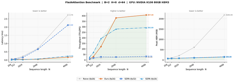 fig 24: benchmarking charts
As you can see in the first graph, our implementation is quite performant than the pytorch fp16 and slightly better than sdpa fp16 on H100. This is probably because triton does autotune at the block level. torch sdpa also does autotuning but that is at the implementation level and tries to find the best implementation. The naive algorithm grows steeply from N=2048 onwards, hitting 2.74ms at N=4096, while our kernel stays nearly flat. This is because the O(\(N^2\)) memory allocation cost is becoming the bottleneck for Naive as the \(N\times N\) matrix grows.
The middle panel, where throughput is being compared, is very interesting. Our kernel reaches 407.40 TFLOPS at N=4096, plateauing sharply after N=1024 which suggests that this is a compute-bound kernel saturating the Tensor Cores. SDPA fp16 reaches 292.09 TFLOPS. Our kernel outperforming SDPA is notable: the autotuner found a tile configuration that maps extremely well to the H100’s Tensor Core dimensions and pipeline depth, while PyTorch’s SDPA backend is dispatching to a cuDNN path that may not be as aggressively tuned for our shapes. When you try the code out change the shapes and benchmark and see if they yield different results. SDPA fp32 and Naive flatline near the bottom at 22–33 TFLOPS indicating that both are memory-bandwidth-bound or compute-limited by fp32 arithmetic, which runs at roughly 1/2 the throughput of fp16 on Tensor Cores.
The last panel is about memory. All tiled implementations stay flat at ~133 MiB regardless of N, confirming O(N) memory scaling. Naive hits 2184 MiB at N=4096 and approaching OOM fast. Even for a small sequence length with B=2, H=8, N=4096, d=64 in fp16 alone (text and small images) of \(2\times 8\times 4096^2\times 2\) bytes \(\approx\) 1 GB. The gap between tiled approach and naive approach will widen quadratically as N grows.
Conclusion#
In this post I have worked through the derivations behind the forward and backward pass of flash attention. If you are running on newer hardware such as Ampere, Hopper or the Blackwell GPUs, then replacing your SDPA attention with flash attention is one of the easiest boosts ups you can do to your LLMs. In the future posts, I will discuss the improvements made to the original flash attention algorithm through flash attention 2, 3, and 4. Thanks for reading this post.
References#
- Dao, Tri, et al. “Flashattention: Fast and memory-efficient exact attention with io-awareness.” Advances in neural information processing systems 35 (2022): 16344–16359.
- Dao, Tri. “Flashattention-2: Faster attention with better parallelism and work partitioning.” arXiv preprint arXiv:2307.08691 (2023).
- Shah, Jay, et al. “Flashattention-3: Fast and accurate attention with asynchrony and low-precision.” Advances in Neural Information Processing Systems 37 (2024): 68658–68685.
- https://superuser.com/questions/695632/why-do-we-need-multiple-levels-of-cache-memory
- CPU cache basics https://dev.to/larapulse/cpu-cache-basics-57ej
- Why do we need multiple levels of cache memory https://superuser.com/questions/695632/why-do-we-need-multiple-levels-of-cache-memory
- L1, L2 and L3 in CPUs https://medium.com/@mike.anderson007/the-cache-clash-l1-l2-and-l3-in-cpus-2a21d61a0c6b
- Why is the cache memory faster than the main memory https://www.reddit.com/r/AskComputerScience/comments/1d68xyi/why_is_the_cache_memory_faster_than_the_main/
- Why is the cache faster than the main memory https://softwareengineering.stackexchange.com/a/234258
- https://cvw.cac.cornell.edu/cuda-intro/gpu-performance-topics/tiling
- https://www.sethweidman.com/blog/cuda_matmul.html
- Z. Ye. UW CSE 599M Spring 2023: ML for ML Systems. From Online Softmax to FlashAttention. https://courses.cs.washington.edu/courses/cse599m/23sp/notes/flashattn.pdf
- https://shreyansh26.github.io/post/2023-03-26_flash-attention/
- FLASH-D: FlashAttention with Hidden Softmax Division https://arxiv.org/html/2505.14201v1
- RijuRekha Sen. IITD. https://www.cse.iitd.ac.in/~rijurekha/col851/flashattention.pdf
- Writing Speed-of-Light Flash Attention for 5090 in CUDA C++. https://gau-nernst.github.io/fa-5090/
- https://peterchng.com/blog/2024/06/26/the-basic-idea-behind-flashattention/
- https://medium.com/data-science-collective/online-softmax-to-flash-attention-and-why-it-matters-9d676e7c50a8
- Milakov, Maxim, and Natalia Gimelshein. “Online normalizer calculation for softmax.” arXiv preprint arXiv:1805.02867 (2018).
- Flash Attention Backpropagation Derivation. https://liyuan24.github.io/writings/attention_backprop.html