 Image 1
LLMs have a large number of parameters in them and this is what makes them so intelligent. But because of this same property they are slow and consume a lot of memory. LLM quantization is a methodology where we reduce the precision of the weights and activations in LLM so that they consume less memory and run faster without a big drop in accuracy. In this post, I will go through various quantization levels such as fp16, bf16, int8 and int4 data types. I will then cover various techniques such as Linear Quantization, Activation Quantization, Block quantization and Quantization Aware Training to understand how better and better quantization levels are achieved in LLMs.
CPUs and GPUs#
First lets through a little bit of the background first.
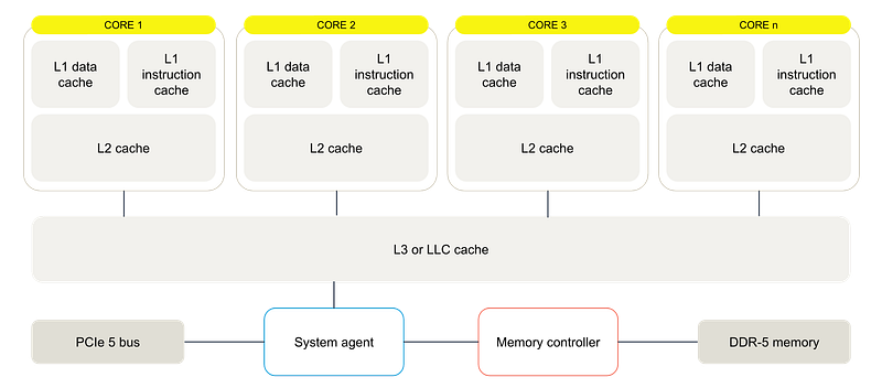 Image 2: CPU architecture. source: CPU vs GPU: What’s best for Machine Learning? | Aerospike
A CPU consists of a few cores optimized for general-purpose sequential serial processing. CPUs are designed to complete tasks with the lowest possible latency and can quickly switch between operations. There is the PCI bus, system agent, memory controller and DDR memory. There is the L3 cache for all the cores. L2 supports individual cores. Separate L1 data cache for data and instructions. If data isn’t found in the cache layers, the CPU retrieves it from the main memory, prioritizing low-latency access for efficiency.
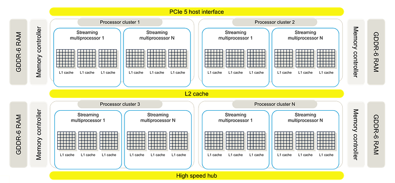 Image 3: GPU architecture source: CPU vs GPU: What’s best for Machine Learning? | Aerospike
In GPUs there are massive number of cores. For example, the latest H100 series from NVIDIA has 16896 cores. Since there are so many cores, there are processor clusters of streaming multiprocessors. Each SM typically has an L1 cache for quick access to instructions. The SMs utilize a shared L2 cache before accessing high-speed memory. Unlike CPUs, GPUs are designed to tolerate higher memory latency. They dedicate more transistors to computation rather than caching. The architecture focuses on keeping the GPU busy with parallel computations despite slower memory access. So the difference is that:
- CPU: Optimized for low-latency, sequential processing.
- GPU: Optimized for high-throughput, parallel processing.
Thus, GPU operations becomes faster if there is less transfer of data and more focus on computation.
Quantization#
As you know the weights in the LLMs as well as the input data is converted to tensors.
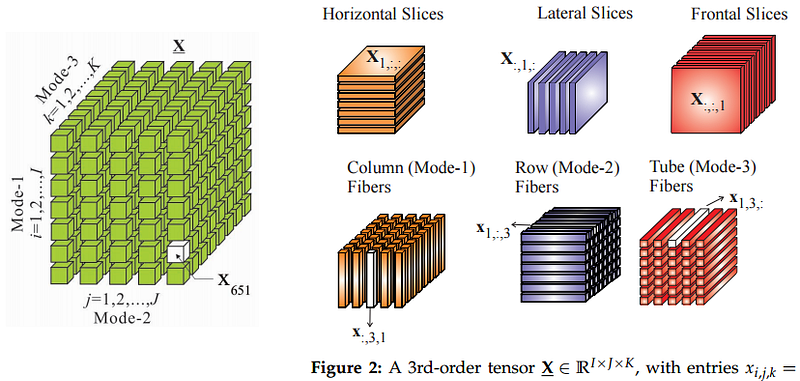 Image 4: Tensors. source: machine learning — Why the sudden fascination with tensors? — Cross Validated
With quantization you convert a model weights and activations from higher precision to lower precision. Quantization makes inference faster because Reducing precision speeds up inference time because it requires less memory, less bandwidth is required for transfer of data and less time for calculations. Traditionally the preferred precision that was utilised was either floating point 32 or floating point 16. Generally, these data is converted from FP16 to INT8. Even INT4 quantization has been quite successful and now efforts are being made so that INT2 is being explored.
Quantization Error#
Before understanding how to check the effect of quantization, let's consider the simplest way to perform quantization. We do this almost every day in our day to day lives — Rounding. In rounding we will just reduce the precision of the weights and activations of the model. In literature this is called the Round to Nearest or RTN approach. Rounding by itself, although looks simple, is a rabbit hole in itself. Ideal characteristics of rounding methods include:
- Rounding should be done by a function or some method such that same input should always mean same output.
- Calculations done with rounding should be close to those done without rounding.
- Rounding should preserve symmetries that already exist between the domain and range. With finite precision (or a discrete domain), this translates to removing bias.
- Generally rounding is done to improve speed so that objective must be achieved.
By default if you create a random matrix in torch it will create the float values in float32 precision. A floating-point variable can represent a wider range of numbers than a fixed-point variable of the same bit width at the cost of precision. As per Wikipedia the range for floating 32 is 3.4028235 \(\times\) \(1^{038}\). In Code 1, if we initiate a 3x3 matrix with float32 and then round the values to float16, then the memory gets halved. Taking the absolute values of the difference and then taking the sum gives the overall error.
Code 1
import torch

mat = torch.rand((3,3))

print(mat)

print('total memory taken', mat.element_size() * mat.nelement())

print('dtype of each data point:', mat[0][0].dtype)

mat_1 = mat.to(dtype=torch.float16)

print(mat_1)

print('total memory taken', mat_1.element_size() * mat_1.nelement())
print('total difference:', (mat - mat_1).abs().sum())

# Output
tensor([[0.2512, 0.7639, 0.4204],
        [0.6266, 0.0650, 0.4428],
        [0.9170, 0.5509, 0.1463]])
total memory taken 36
dtype of each data point: torch.float32
tensor([[0.2512, 0.7637, 0.4204],
        [0.6265, 0.0650, 0.4429],
        [0.9170, 0.5508, 0.1462]], dtype=torch.float16)
total memory taken 18
total difference: tensor(0.0007)
Running Code 1 may result in different matrices and different quantization error every time you run it because the matrices are initialised randomly.
Quantization Error is the difference between the original values of the tensor and its quantized values. No matter whatever number you want to identify. In many cases you are quantizing in any case for example in case of irrational numbers because of the inherent limitations of computer systems. And then there is additional loss of precision because you want to expand your range of numbers that you want to represent. So here you can understand that if you want to give form to knowledge you are in any case bringing in some loss in information.
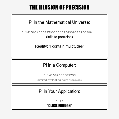 Image 5: The illusion of exactness
So, the question becomes what an “ACCEPTABLE” loss of precision and is my ideal scenario would be what the accuracy on your domain is and on your benchmark dataset, but if you are creating a general model in which case this is probably not there, maybe quantization error is fine. In the next section, we will go through another popular data type bfloat16 and then compare the Quantization Error between rounding to fp16 and bf16 and see which one is closer to fp32 values.
Brain Float 16#
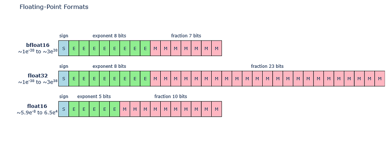 Image 6: bfloat16 range comparison
For deep learning applications google came up with this format called brain float 16 or bfloat16 which has the same number of bits as float16 but the dynamic range is the same as float32 because exponent size of bfloat16 floating point is the same as float32. As per available literature Training behavior with bfloat16 setting is more robust and is less prone to underflows, overflows, or any other numerical instability during training compared to training with pure float32 dtype. So, in many ways bfloat is really useful if you are doing training. You can go through the code in this colab.
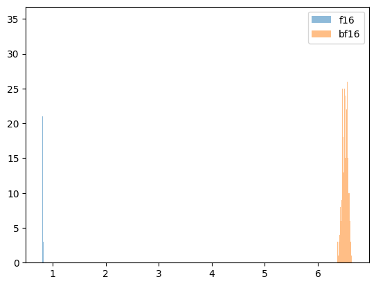 Image 7: difference between float16 and bfloat16
Interestingly similar to the errors that we got from f16 quantization, we check the quantization error for bf16 as well. To compare we take the sum of the absolute values of the errors. The error for bf16 is more. I took 1000 random tensors. and then took the distribution of the errors. If the matrix is small then the bf16 errors are wider, but if we increase the size of the matrix then the bf16 errors become more pronounced and separated out.
Even though bf16 is not enough with todays quantization needs, you will be able to load a decent llm such as llama3 8b model on colab which has around 16gb gpu memory. The unquantized one was giving memory error but using bf16 total around 12gb is being used.
Code 2
from transformers import AutoTokenizer, AutoModelForCausalLM
import torch

model_id = "meta-llama/Meta-Llama-3-8B-Instruct"

tokenizer = AutoTokenizer.from_pretrained(model_id)
model = AutoModelForCausalLM.from_pretrained(
    model_id,
    torch_dtype=torch.bfloat16, # without this it will give memory error in colab
    device_map="auto",
)
In terms of quantization, based on what you are quantizing, there are two types of quantization: model quantization and activation quantization. Since in bf16 you are just reducing the precision of the model weights from fp32 to bf16, this is a type of model quantization.
Linear Quantization#
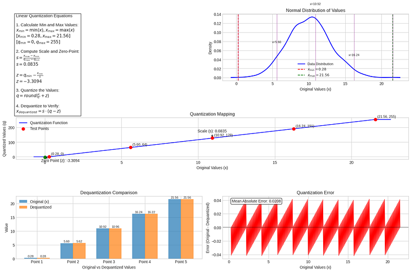 Image 8: showcasing linear quantization with z and s values
In linear quantization you find the zero point and scale values assuming the unquantized values follow a normal distribution. You can do this for both the model weights and the activations. If you are finding the zero point then this is asymmetric else you can just define the scale in which case this will be called symmetric. As you can see in equations 1–6, you scale the total range to fit as per the range of the quantized values and so this is also called affine quantization. The zero-point is there to ensure that zero in the floating-point range is accurately represented by an integer. This maintains numerical accuracy and stability, especially for values close to zero. Then you quantize whatever values comes. The rounding operation ensures that the final result is a discrete integer, suitable for storage and computation in lower precision formats. During inference, the dequantized values are used for calculations to achieve higher precision, although only the quantized weights are stored.
You can perform linear quantization on the models using optimum quanto library from huggingface. I am taking model “meta-llama/Llama-3.2–1B-Instruct” and loading it is taking 4714 MB of memory in float32. You can check this by printing the dtype of the weights. I can then quantize it using the quanto library and post quantization the memory actually increases to 5716 MB. Code 3 shows the print of the same decoder layer from unquantized to quantized. Observe the the Linear class has been changed to QLinear.
Code 3
# Original float32 weights
LlamaDecoderLayer(
  (self_attn): LlamaSdpaAttention(
    (q_proj): Linear(in_features=2048, out_features=2048, bias=False)
    (k_proj): Linear(in_features=2048, out_features=512, bias=False)
    (v_proj): Linear(in_features=2048, out_features=512, bias=False)
    (o_proj): Linear(in_features=2048, out_features=2048, bias=False)
    (rotary_emb): LlamaRotaryEmbedding()
  )
  (mlp): LlamaMLP(
    (gate_proj): Linear(in_features=2048, out_features=8192, bias=False)
    (up_proj): Linear(in_features=2048, out_features=8192, bias=False)
    (down_proj): Linear(in_features=8192, out_features=2048, bias=False)
    (act_fn): SiLU()
  )
  (input_layernorm): LlamaRMSNorm((2048,), eps=1e-05)
  (post_attention_layernorm): LlamaRMSNorm((2048,), eps=1e-05)
)

# Quantized weights
LlamaDecoderLayer(
  (self_attn): LlamaSdpaAttention(
    (q_proj): QLinear(in_features=2048, out_features=2048, bias=False)
    (k_proj): QLinear(in_features=2048, out_features=512, bias=False)
    (v_proj): QLinear(in_features=2048, out_features=512, bias=False)
    (o_proj): QLinear(in_features=2048, out_features=2048, bias=False)
    (rotary_emb): LlamaRotaryEmbedding()
  )
  (mlp): LlamaMLP(
    (gate_proj): QLinear(in_features=2048, out_features=8192, bias=False)
    (up_proj): QLinear(in_features=2048, out_features=8192, bias=False)
    (down_proj): QLinear(in_features=8192, out_features=2048, bias=False)
    (act_fn): SiLU()
  )
  (input_layernorm): LlamaRMSNorm((2048,), eps=1e-05)
  (post_attention_layernorm): LlamaRMSNorm((2048,), eps=1e-05)
)
Why more memory for the quantized model? Probably because the library is storing the weights as well as the quantized and scale values as I have called the freeze method in the code. As per the documentation the weights are dynamically quantized, hence you need to call freeze to have them beforehand. When we print one of the mlp gate proj weight we can see Code 4. You can see that the weights and the scale values are given.
Code 4
<class 'optimum.quanto.tensor.weights.qbytes.WeightQBytesTensor'>(tensor([[ 54, -26, -29,  ...,   7,  57,  76],
        [-19,  44,   3,  ..., -54, -30,   5],
        [-41, -15,   0,  ...,  -9, -19, -45],
        ...,
        [ 34, -40, -33,  ...,  50, -74, -24],
        [ -4, -19,   2,  ...,  -6,  11, -24],
        [-41,   9,  15,  ..., -21, -12,  12]], dtype=torch.int8), scale=tensor([[0.0005],
        [0.0005],
        [0.0006],
        ...,
        [0.0006],
        [0.0006],
        [0.0006]]), dtype=torch.float32)
And if you check with the original weights the attention weights are the same. But if you check the mlp weights there is a difference there.
before quantization: 0.026000977, -0.012329102, -0.013977051, \(\dots\)
after quantization: 0.025951955, -0.012495386, -0.013937162, \(\dots\)
Activation Quantization#
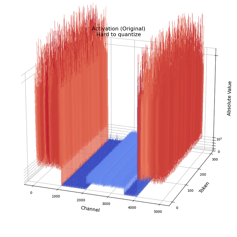 Image 9: Outliers in activations
Now why to limit quantization to only the weights when you can do activation quantization as well. Although activation quantization looks like it has better promise it is harder to achieve. Why? Because unlike weights, which are static (constant) once the model is trained, activations are dynamic. This means that activations change with each input to the network, making their range harder to predict.
LLMs are notoriously difficult to quantize due to the outliers in the activations. In case of weights, the weight distribution is quite uniform and flat, which is easy to quantize. From the analysis done in the smoothquant paper:
- Outliers make activation quantization difficult. The scale of outliers in activations is ∼\(100\times\) larger than most of the activation values. In the case of per-tensor quantization, the large outliers dominate the maximum magnitude measurement, leading to low effective quantization bits/levelsfor non-outlier channels. For non-outlier channels, the effective quantization levels would be very small (2–3), leading to large quantization errors.
- Outliers persist in fixed channels. Outliers appear in a small fraction of the channels. If one channel has an outlier, it persistently appears in all tokens. The variance amongst the channels for a given token is large (the activations in some channels are very large, but most are small), but the variance between the magnitudes of a given channel across tokens is small (outlier channels are consistently large).
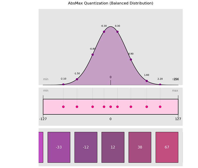 Image 10
For activation quantization you can understand that you will need a calibration data to compute the activation quantization parameters. For example in optimum quanto library, if you pass the option to perform activation quantization then you need to provide some calibration data. The library will then track maximum absolute values per channel during forward passes. Use these absmax values to derive per-channel scaling factors and apply them during quantization.
Code 5
from optimum.quanto import quantize, qint8
from optimum.quanto import Calibration

quantize(model, weights=qint8, activations=qint8)
with Calibration(momentum=0.9):
    model(samples)
Dynamic Quantization#
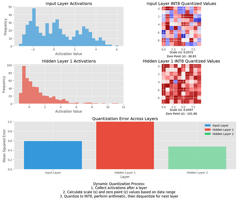 Image 11
In the previous section, we discussed an example of static quantization where we calculate the zeropoint and scale prior to inference using a calibration dataset. In contrast we can do dynamic quantization as well where we calculate the parameters during runtime and not utilize a calibration dataset.
Steps for dynamic quantization:
- After data passes a hidden layer, its activations are collected:
- This distribution of activations is then used to calculate the zeropoint (z) and scale factor (s) values dynamically based on the data range observed at runtime. This ensures that the scale factor is “tuned” so that as much signal as possible about each observed dataset is preserved.
- The process is repeated each time data passes through a new layer. Therefore, each layer has its own separate z and s values and therefore different quantization schemes.
The model parameters are known during model conversion and they are converted ahead of time and stored in INT8 form. Arithmetic in the quantized model is done using vectorized INT8 instructions. Accumulation is typically done with INT16 or INT32 to avoid overflow. This higher precision value is scaled back to INT8 if the next layer is quantized or converted to FP32 for output.
Dynamic quantization is relatively free of tuning parameters which makes it well suited to be added into production pipelines. In general, dynamic quantization tends to be a bit more accurate since it only attempts to calculate the s and z values per hidden layer. However, it might increase compute time as these values need to be calculated.
Block Quantization#
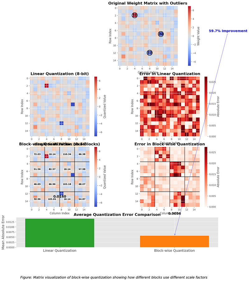 Image 12
As we have discussed till the main problem with linear quantization is that Outliers can have a disproportionate impact on scaling: the full range of the lower-precision data type isn’t used effectively — which lowers the quantized model’s accuracy.
The solution to this is quantizing in blocks, whereby weights are divided into groups of 64 or 128, for example, according to their value. Each block is then quantized individually to mitigate the effect of outliers and increase precision.
Something to factor in, however, is that while an LLM’s weights and activations will be quantized to reduce its size, they will be dequantized at inference time, so the necessary computations during forward and backward propagation can be performed with a higher-precision data type.
This means that the scaling factors for each block must also be stored. Consequently, the more blocks that are used during the quantization process, the higher the accuracy — but the higher the number of scaling factors that must also be saved.
The famous GGUF quantization uses this block methodology to quantize the LLMs. As per their the comments in that discussion:
Quantization Aware Training#
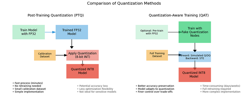 Image 13
There are two ways you can perform quantization: Post training quantization where we take an already trained model and perform quantization on it. The methods that we have been discussing before are post training quantization methods. Post-training quantization (PTQ) schemes quantize models in a greedy fashion. Specifically, these algorithms usually optimize an auxiliary loss function representing the distance between the quantized and unquantized operands and parameters in the network. The optimization is applied on a per-layer basis using only a few training samples, known as the calibration set. Although these approaches are computationally inexpensive, they often decrease network
accuracy.
There are various recipes to perform QAT, from starting with an untrained model to starting with a pretrained model. All recipes change the training regimen to include the quantization error in the training loss by inserting fake-quantization operations into the training graph to simulate the quantization of data and parameters. These operations are called ‘fake’ because they quantize the data, but then immediately dequantize the data so the operation’s compute remains in float-point precision. This trick adds quantization noise without changing much in the deep-learning framework.
In the forward-pass, you fake-quantize the floating-point weights and activations and use these fake-quantized weights and activations to perform the layer’s operation. In the backward pass, you use the weights’ gradients to update the floating-point weights. To deal with the quantization gradient, which is zero almost everywhere except for points where it is undefined, you use the (straight-through estimator (STE), which passes the gradient as-is through the fake-quantization operator. When the QAT process is done, the fake-quantization layers hold the quantization scales that you use to quantize the weights and activations that the model is used for inference.
Lets suppose we want to binarize the activations of a layer using the following function.
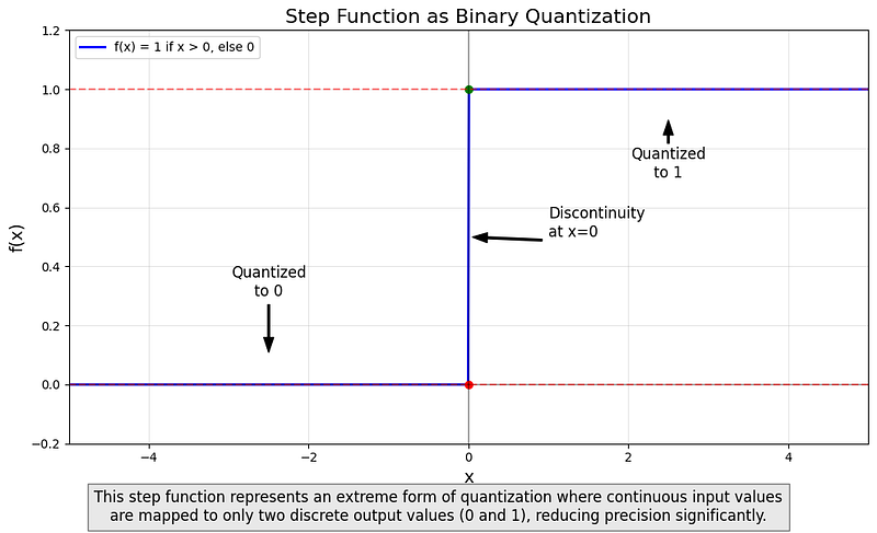 Image 14
This function will return 1 for every value that is greater than 0 otherwise it will return 0. This is similar to quantization operation since you are reducing the precision of the output activations.
As mentioned earlier, the problem with this function is that its gradient is zero. To overcome this issue we will use a straight-through estimator in the backward pass.
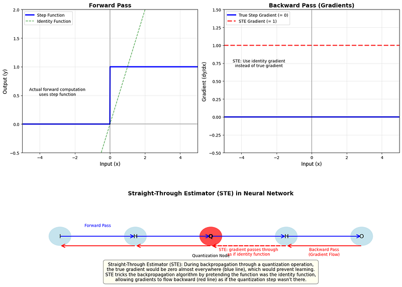 Image 15
A straight-through estimator is exactly what it sounds like. It estimates the gradients of a function. Specifically, it ignores the derivative of the threshold function and passes on the incoming gradient as if the function was an identity function.
QLoRA#
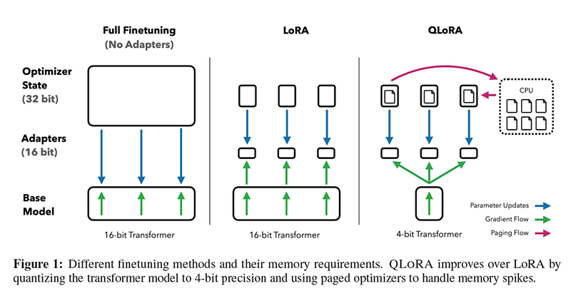 Image 16: Image source QLoRA paper
Current popular methods in QAT is QLoRA where we finetune the performance of LLMs to bring up the loss in accuracy. I have talked about efficient finetuning of transformers using QLoRA in this video. Check it out.
The steps for the algorithm as discussed in the paper are discussed below.
The weights of pretrained neural networks are assumed to follow a zero-centered normal distribution, meaning they are distributed around a central value of zero. The weights are normalized in the range of [-1, 1]. This normalization is achieved by diving each weight by absmax algorithm which we discussed before. By normalizing the input data, we are distributing the weights around zero and the less bits are required to store the exponential data of a tensor/weight parameter.
The exact values for NF4 data type (16 bins) are as follows: These values are there in the paper.
[-1.0, -0.6961928009986877, -0.5250730514526367, -0.39491748809814453, -0.28444138169288635, -0.18477343022823334, -0.09105003625154495, 0.0, 0.07958029955625534, 0.16093020141124725, 0.24611230194568634, 0.33791524171829224, 0.44070982933044434, 0.5626170039176941, 0.7229568362236023, 1.0]
Next block quantization is done. We have already discussed about block quantization. Block-wise quantization divides input tensors into smaller blocks and quantizes each block independently which reduces the problem of outlier. In this process we split the input tensor into chunks, and each chuck is quantized independently with each having their own quantization constant (total bins of datatype/absolute max tensor). Even with outliers we get much higher quantization precision and stability with block wise k-bit quantization by confining outliers to blocks. They flatten the weights and do the absmax normalization after dividing into equal sized blocks. You take each block and divide to 16 bins and then map to the closest NF4 level.
Next is double quantization. Double Quantization (DQ) is a process of quantizing the quantization constants for additional memory savings. QLoRA quantizes weights in blocks of 64, and while this facilitates precise 4-bit quantization, you also have to account for the scaling factors of each block — which increases the amount of memory required. DQ addresses this issue by performing a second round of quantization on the scaling factors for each block. The 32-bit scaling factors are compiled into blocks of 256 and quantized to 8-bit. Consequently, where a 32-bit scaling factor for each block of previously added 0.5 bits per weight, DQ brings this down to only 0.127 bits. If you argue that is this really required? Doesn't it seem insignificant, then actually when combined in a 65B LLM this saves 3 GB of memory.
The storage part is also interesting and worth mentioning. This part depends on the library and is not actually mentioned in the paper. It turns out the author of bitsandbytes which is the official implementation of qlora converts the 4-bit values into 8-bit by packing two 4 bit values into a single 8-bit value, this results ofcourse, in a different shape for the quantized tensor. This is because PyTorch does not support 4-bit data types and the smallest type it supports is 8-bits. The reason it uses an 8-bit integer format and not an 8-bit floating point format FP8 is due to the lack of native support for FP8 in PyTorch. The packing operation is exactly what Pytorch’s new data type ‘quantized 4-bit integer’ torch.quint4x2 does as well, as you can see in the documentation.
If code is what you connect with more, Code 6 is the code for the above description.
Code 6
import torch

NF4_quant_levels = torch.tensor([-1.0, -0.6961928009986877, -0.5250730514526367, -0.39491748809814453, -0.28444138169288635, -0.18477343022823334, -0.09105003625154495, 0.0, 0.07958029955625534, 0.16093020141124725, 0.24611230194568634, 0.33791524171829224, 0.44070982933044434, 0.5626170039176941, 0.7229568362236023, 1.0])

#  binary representation of uint4 values (used 4-bit binaries instead of decimals for illustration purposes)
nf4_quant_4bit = torch.tensor([0b0000, 0b0001, 0b0010, 0b0011, 0b0100, 0b0101, 0b0110, 0b0111, 0b1000, 0b1001, 0b1010, 0b1011, 0b1100, 0b1101, 0b1110, 0b1111])

# generated tensor of [5, 4] shape
W = torch.tensor([[ 0.4767, -0.2921,  0.0787, -0.1018],
                  [-0.3453,  0.3834, -0.0107, -0.4692],
                  [-0.4072, -0.2996, -0.4942, -0.2640],
                  [ 0.0125,  0.2962,  0.3123, -0.4705],
                  [-0.1982, -0.1545,  0.3358, -0.4086]])

flat_W = W.flatten()

# normalize the tensor using absmax to fit within [-1, 1]
max_val = flat_W.abs().max()
normalized_W = flat_W / max_val

# map each input value to its nearest quantization level - then to its 4-bit binary representation
quantized_W_4bits = torch.zeros(normalized_W.shape, dtype=torch.int)
for i, val in enumerate(normalized_W):
    closest_level = torch.argmin(torch.abs(NF4_quant_levels - val)) # get the index of closest quantization level
    quantized_W_4bits[i] = nf4_quant_4bit[closest_level]

print(quantized_W_4bits)
# Output: [15,  2,  9,  5,  1, 14,  7,  0,  1,  2,  0,  2,  7, 13, 13,  0,  3,  4, 14,  1]

packed_W_8bits = []
for i in range(0, len(quantized_W_4bits), 2):
    # Courtesy of https://www.geeksforgeeks.org/store-two-numbers-in-one-byte-using-bit-manipulation/
    # take each pair of 4-bit values in quantized_W_4bits and combine them into packed_W_8bits by shifting
    # the first 4 bits to the left using the left shift operator '<<' and combining them using the OR | operation
    result = (quantized_W_4bits[i] << 4) & 0xff
    result =  result | quantized_W_4bits[i + 1]
    packed_W_8bits.append(result)

# set it as torch.uint8
packed_W_8bits = torch.tensor(packed_W_8bits, dtype=torch.uint8)

print(packed_W_8bits)
# Output: tensor([242, 149,  30, 112,  18,   2, 125, 208,  52, 225], dtype=torch.uint8)
Code reference: https://manalelaidouni.github.io/4Bit-Quantization-Models-QLoRa.html
Final thoughts and workflow#
If after all this information you are confused about which quantization algorithm to choose and how to go about it here is a nice flowchart that is derived from the steps mentioned in the huggingface documentation.
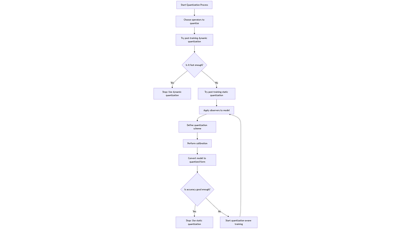 Image 17
To effectively quantize a model to int8, the steps to follow are:
- Choose which operators to quantize. Good operators to quantize are the one dominating it terms of computation time, for instance linear projections and matrix multiplications.
- Try post-training dynamic quantization, if it is fast enough stop here, otherwise continue to step 3.
- Try post-training static quantization which can be faster than dynamic quantization but often with a drop in terms of accuracy. Apply observers to your models in places where you want to quantize. implies defining which quantization scheme to use.
- Perform calibration.
- Convert the model to its quantized form: the observers are removed and the float32 operators are converted to their int8 coutnerparts.
- Evaluate the quantized model: is the accuracy good enough? If yes, stop here, otherwise start again at step 3 but with quantization aware training this time.
Concerned about the current job market? Need career or project guidance? Lets connect on linkedin or topmate.
|  Image 18 |  Image 19 |
References:#
- CPU vs GPU: https://aerospike.com/blog/cpu-vs-gpu/
- Number of cores in GPU: https://en.wikipedia.org/wiki/Hopper_(microarchitecture)#H100_accelerator_and_DGX_H100
- FP8: https://arxiv.org/abs/2303.17951
- Tensors: https://www.avni.sh/posts/linear-algebra/tensors/
- Deepseek: https://www.youtube.com/watch?v=2IRLJbTXWmI
- Floating Point Format: https://en.wikipedia.org/wiki/Single-precision_floating-point_format
- Int2: https://arxiv.org/abs/2306.08162
- Why does model quantization speed up inference discussion: https://www.reddit.com/r/learnmachinelearning/comments/zgzh6r/whyhow_does_model_quantization_speed_up_inference/
- Datacamp on Quantization: https://www.datacamp.com/tutorial/quantization-for-large-language-models
- Block Quantization: https://www.youtube.com/watch?v=IxrlHAJtqKE
- Rounding: https://en.wikipedia.org/wiki/Rounding
- Bfloat 16: https://en.wikipedia.org/wiki/Bfloat16_floating-point_format
- Weight and Activation Quantization showcase: https://www.catalyzex.com/paper/joint-training-of-low-precision-neural
- Linear Quantization Pytorch Blog: https://pytorch.org/blog/quantization-in-practice/
- LLM.int8 Tim Dettmers paper: https://arxiv.org/pdf/2208.07339
- Zero Point Quantization: https://medium.com/@luis.vasquez.work.log/zero-point-quantization-how-do-we-get-those-formulas-4155b51a60d6
- SmoothQuant and challenges with outliers: https://arxiv.org/html/2211.10438v7
- Outliers: https://aakashvarma.substack.com/p/smoothquant
- Calibration implementation using AbsMax: https://github.com/huggingface/optimum-quanto/blob/main/optimum/quanto/calibrate.py#L37
- maartengrootendorst blog: https://newsletter.maartengrootendorst.com/p/a-visual-guide-to-quantization
- symbl.ai blog: https://symbl.ai/developers/blog/a-guide-to-quantization-in-llms/
- Block Quantization: https://arxiv.org/pdf/2110.02861
- Quantization in GGUF: https://github.com/ggerganov/llama.cpp/discussions/4068#discussioncomment-7566463
- Dynamic Quantization: https://arxiv.org/pdf/2306.02316
- Pytorch Dynamic Quantization: https://pytorch.org/tutorials/recipes/recipes/dynamic_quantization.html
- Dynamic Quantization On Bert: https://colab.research.google.com/github/pytorch/tutorials/blob/gh-pages/_downloads/dynamic_quantization_bert_tutorial.ipynb
- Quantization Aware Training Methodology: https://arxiv.org/abs/2411.11038
- Straight Through Estimator: https://arxiv.org/pdf/1308.3432
- Yoshua Bengio: https://en.wikipedia.org/wiki/Yoshua_Bengio
- STE Implementation: https://hassanaskary.medium.com/intuitive-explanation-of-straight-through-estimators-with-pytorch-implementation-71d99d25d9d0
- QLoRA: https://arxiv.org/pdf/2305.14314
- QLoRA Explained: https://medium.com/@dillipprasad60/qlora-explained-a-deep-dive-into-parametric-efficient-fine-tuning-in-large-language-models-llms-c1a4794b1766
- WanDB on QLoRA: https://wandb.ai/sauravmaheshkar/QLoRA/reports/What-is-QLoRA---Vmlldzo2MTI2OTc5
- Manal El Aidouni blog: https://manalelaidouni.github.io/4Bit-Quantization-Models-QLoRa.html