LLM Quantization Techniques

Image 1

This is the second part of the series on LLM Quantization. In the previous blog post we discussed about the theory behind LLM Quantization such as Linear Quantization, Activation Quantization and Quantization Aware Training [blog and video]. In this post, we will discuss about the various specific algorithms and the associated libraries such as GPTQ, AWQ, GGUF, HQQ and BitNet.

SetUp#

Dataset#

Before moving into discussing about the different libraries, lets start with developing some common code that can be utilised for benchmarking.

Code 1

# call notebook login
from huggingface_hub import notebook_login
notebook_login()

# install required libraries
!pip install -q datasets
!pip install -q nvidia-ml-py3

# load the dataset.
from datasets import load_dataset
dataset = load_dataset('semeru/code-text-python', split='test[:100]')
print(f'{len(dataset)=}')

# save the dataset in a file
with open('dataset.txt', 'w') as fw:
  for line in dataset['original_string']:
    fw.write(f'{line}\n')

In Code 1, we login into huggingface. This assumes that you are running in notebook hence we are using the notebook_login method. Install the library datasets for loading our favorite dataset and and nvidia-ml-py3 to get memory usage. Load the dataset semeru/code-text-python. Seeing that the code completion use case is quite popular for LLMs these days, so I thought of benchmarking using a code dataset. I am using just 100 samples to make the code run faster in general but you should probably use more samples and representative of your use case.

Calculate Perplexity#

Code 2

import torch
from tqdm import tqdm
device = torch.device('cuda' if torch.cuda.is_available() else 'cpu')

def calculate_perplexity(model, tokenizer, dataset, modelname):
  """
  Calculate the perplexity of a language model on a given dataset.

  """
  max_length = 100
  stride = 50
  encodings = tokenizer("\n\n".join(dataset['original_string']), return_tensors="pt")
  seq_len = encodings.input_ids.size(1)

  nll_sum = 0.0
  n_tokens = 0
  prev_end_loc = 0
  for begin_loc in tqdm(range(0, seq_len, stride)):
      end_loc = min(begin_loc + max_length, seq_len)
      trg_len = end_loc - prev_end_loc  # may be different from stride on last loop
      input_ids = encodings.input_ids[:, begin_loc:end_loc].to(device)
      target_ids = input_ids.clone()
      target_ids[:, :-trg_len] = -100

      with torch.no_grad():
          outputs = model(input_ids, labels=target_ids)

          # loss is calculated using CrossEntropyLoss which averages over valid labels
          # N.B. the model only calculates loss over trg_len - 1 labels, because it internally shifts the labels
          # to the left by 1.
          neg_log_likelihood = outputs.loss

      # Accumulate the total negative log-likelihood and the total number of tokens
      num_valid_tokens = (target_ids != -100).sum().item()  # number of valid tokens in target_ids
      batch_size = target_ids.size(0)
      num_loss_tokens = num_valid_tokens - batch_size  # subtract batch_size due to internal label shift
      nll_sum += neg_log_likelihood * num_loss_tokens
      n_tokens += num_loss_tokens

      prev_end_loc = end_loc
      if end_loc == seq_len:
          break

  avg_nll = nll_sum / n_tokens  # average negative log-likelihood per token
  ppl = torch.exp(avg_nll)

  print()
  print(f'Perplexity for model name {modelname}: {ppl.detach().cpu().numpy():.4f}')

  return ppl

Code 2 is to calculate the perplexity for a specific model and dataset. Most of the code for this is taken from the huggingface documentation. Here we are passing the tokens via the model and then taking the average of the loss. Finally, we take the exp of the average loss.

Generate response#

Code 3

def generate_response(model, tokenizer):
  messages = [
      {"role": "system", "content": "You are a pirate chatbot who always responds in pirate speak!"},
      {"role": "user", "content": "Who are you?"},
  ]

  input_ids = tokenizer.apply_chat_template(
      messages,
      add_generation_prompt=True,
      return_tensors="pt"
  ).to(model.device)

  terminators = [
      tokenizer.eos_token_id,
      tokenizer.convert_tokens_to_ids("<|eot_id|>")
  ]

  outputs = model.generate(
      input_ids,
      max_new_tokens=256,
      eos_token_id=terminators,
      do_sample=True,
      temperature=0.6,
      top_p=0.9,
  )
  response = outputs[0][input_ids.shape[-1]:]
  return tokenizer.decode(response, skip_special_tokens=True)

Code 3 defines a common function for generating the response based on the model and tokenizer. We create a dictionary based on the chat template and create input ids based on it. We pass the input ids via the model to generate the outputs. Temperature is kept at 0.6, top p is 0.9 and max new tokens is 256. We take the top output and remove the input ids to get the generated tokens. These are then decoded to get the text.

Memory Utilization#

Code 4

import nvidia_smi

def get_gpu_memory_utilisation():
  nvidia_smi.nvmlInit()

  deviceCount = nvidia_smi.nvmlDeviceGetCount()
  for i in range(deviceCount):
      handle = nvidia_smi.nvmlDeviceGetHandleByIndex(i)
      info = nvidia_smi.nvmlDeviceGetMemoryInfo(handle)
      print("Device {}: {}, Memory : ({:.2f}% free): {}(GB total), {} (GB free), {} (GB used)".format(i, nvidia_smi.nvmlDeviceGetName(handle), 100*info.free/info.total, info.total / (1024**3), info.free / (1024**3), info.used / (1024**3)))

  nvidia_smi.nvmlShutdown()

Code 4 defines a common function to get the gpu memory utilization. For this we are using the nvidia-smi library that we installed earlier.

Optimum Quanto#

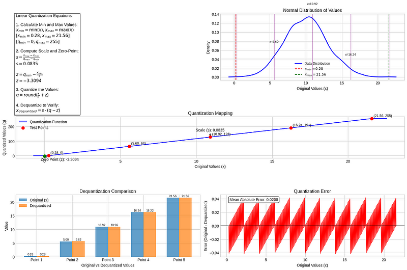Image 2: Linear Quantization | Image by Author

We will start with quantization and how to do linear quantization using OptimumQuanto. We have discussed about OptimumQuanto in the previous video as well. This is a fairly new library with release in October 2023. Because this library directly implements linear quantization which we have talked about extensively in the previous blog we are discussing this first.

LLM Quantization Explained. Shrinking AI models from feast to fit… | by joydeep bhattacharjee | Medium

Code 5

!pip install -q optimum-quanto

from transformers import AutoModelForCausalLM, AutoTokenizer
model_name = "meta-llama/Llama-3.2-1B-Instruct"
model = AutoModelForCausalLM.from_pretrained(model_name, low_cpu_mem_usage=True)
tokenizer = AutoTokenizer.from_pretrained(model_name)

from optimum.quanto import quantize, qint8
quantize(model, weights=qint8)

text = "tell me a joke about LLM quantization."
inputs = tokenizer(text, return_tensors="pt")
outputs = model.generate(**inputs, max_new_tokens=100)
print(tokenizer.decode(outputs[0], skip_special_tokens=True))

In Code 5, we pass the model id and the tokenizer using the classes AutoModelForCausalLM and AutoTokenizer classes. We get copy the model id from huggingface. We use the quantize method from the library to quantize the model. For this we pass the quantization type for the weights and the activations and based on this only the weights or both weights and activations will be quantized. If you are doing activation quantization then you will need to run it through a calibration data but it was not happening in colab and was getting killed due to memory error so not showing the code here but you can check out the method in their official github page.

BitsAndBytes#

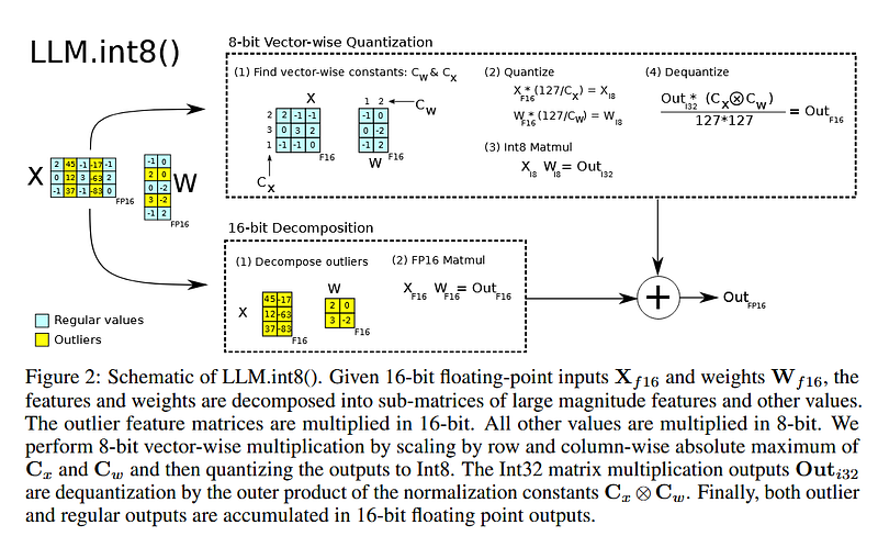Image 3: image from paper: https://arxiv.org/abs/2208.07339

Next, we will start with bits and bytes. This paper came out in June 2022. It started out with the research regarding quantization at hugging phase and its FP8 implementation. The research was primarily done by Tim Dattmers, who is a big name in the quantization community. In the last 10 odd years, he has done a lot of research with big names like Int8 quantization and qlora. In the LLM.int8 paper, they basically studied the effect of outliers in the transformers and did mixed precision decomposition for better output. They implemented this using blockwise quantization, which we have also seen in the previous video. This is for the 8-bit quantization. For moving to 4-bit quantization, qlora was introduced in bits and bytes.

Code and Benchmarking#

Code 6

!pip install -q transformers accelerate bitsandbytes

from transformers import AutoTokenizer, AutoModelForCausalLM, BitsAndBytesConfig
import torch

quantization_config = BitsAndBytesConfig(load_in_8bit=True)
model_id = "meta-llama/Meta-Llama-3-8B-Instruct"
tokenizer = AutoTokenizer.from_pretrained(model_id)
model = AutoModelForCausalLM.from_pretrained(
    model_id,
    quantization_config=quantization_config,
    device_map="auto",
)
get_gpu_memory_utilisation()
print('response from model:', generate_response(model, tokenizer))
calculate_perplexity(model, tokenizer, dataset, model_id)
# Output
'''
Device 0: b'Tesla T4', Memory : (40.83% free): 15.0(GB total), 6.1251220703125 (GB free), 8.8748779296875 (GB used)
response from model: Arrrr, me hearty! Me name be Captain Chatbot, the scurviest pirate to ever sail the Seven Seas! I be a swashbucklin' chatbot, here to regale ye with tales o' adventure, answer yer questions, and maybe even steal yer treasure... er, I mean, yer attention! So hoist the colors, me hearty, and let's set sail fer a chat like no other!
99%|█████████▉| 396/398 [01:14<00:00,  5.29it/s]
Perplexity for model name meta-llama/Meta-Llama-3-8B-Instruct: 5.3226
'''

In Code 6, to quantize and load the model in 8bit using bitsandbytes we create the quantization config using the BitsAndBytesConfig class and then pass this config when creating the model using AutoModelForCausalLM. We can then get the gpu memory utilisation and perplexity using the functions we had defined earlier.

Code 7

      Metrics    UnQ     Q
0      Memory  12.41  8.87
1    Time (m)  10.90  1.40
2  Perplexity   5.28  5.32

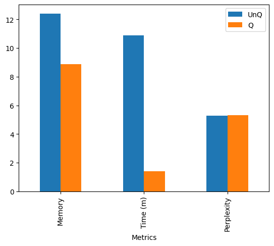Image 4: Bitsandbytes comparison

If we now plot the comparison graphs from Code 7, perplexity is slightly degraded between unquantized and quantized model from 5.28 to 5.32 which is less than 1% degradation. While cumulative time improves from 10.9m to 1.4m or 87% improvement and memory improves from 12.41 GB to 8.87 Gb which is 28.5% improvement. So just moving from bf16 to int8 gives a lot of improvement without much change in perplexity

GPTQ#

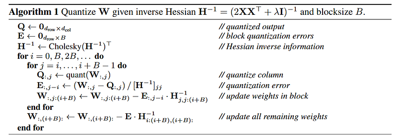Image 5: GPTQ algorithm from paper: https://arxiv.org/abs/2210.17323

Now let’s talk about the GPTQ algorithm. This algorithm was submitted in 31 October 2022. GPTQ is a post-training quantization method to make the model smaller with a calibration dataset. For every layer L in the network, we want to find a quantized version \(\hat{W}\) of the original weights \(W\). This is called the layer-wise compression problem, shown in equation 1.

Concretely, as shown in equation 1, if \(W\) is the weights of the linear layer and \(x\) is the input corresponding to a small set of m data points running through the network, then the objective is to find a matrix of quantized weights \(\hat{W}\) which minimizes the squared error relative to the full precision layer output. Hence, we can say that we are finding the \(\hat{W}\) for the argmin of the squared error of the outputs where \(x\) is a small calibration dataset of activations.

So GPTQ has several key insights to make it more effective than simpler quantization approaches.

1. First is processes weights in order of importance, focusing on the most impactful weights first.
2. Second, it uses the Hessian matrix to understand the complex interaction between different weights.
3. Third, it quantizes weights column by column in blocks for efficiency.
4. And most importantly, it redistributes quantization errors to minimize their impact on model performance.

Role of Hessian in GPTQ#

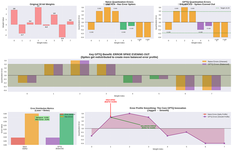Image 6: image by author

When we quantize the original weights in 32 bit to 4-bit representation, each weight gets rounded to the nearest available value in our 4-bit representation. This introduces quantization errors, the differences between the original and the quantized values. In naive quantization, these errors accumulate and cause significant performance degradation. The brilliance of GPTQ is that it doesn’t just accept these errors, it redistributes them to minimize their impact. This is the essence of GPTQ — it doesn’t just minimize total error, it strategically redistributes errors to prevent any weight from becoming a performance bottleneck due to excessive quantization error.

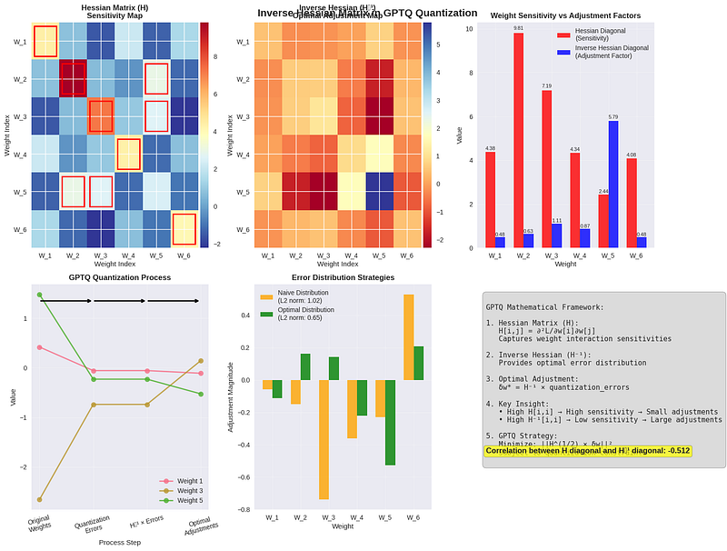Image 7: GPTQ framework | image by author

The secret sauce of GPTQ is the Hessian matrix. The Hessian captures how the model’s error changes with respect to the weight changes, essentially a sensitivity map showing which weights are most important. The inverse of the Hessian tells us how to optimally distribute quantization errors across the weights. Specifically, we want to make larger adjustments to weights that have less impact on the model output.

In the top row of Image 7, you can see a heatmap showing the second-order derivatives matrix that captures how model error changes with weight perturbations. Red boxes highlight areas of high sensitivity where weights strongly interact and affect model output. In the second panel of Image 7, the inverted sensitivity map that reveals where larger quantization adjustments can be safely made. This matrix is the “secret sauce” that tells us how to optimally distribute errors. The bar chart comparing diagonal elements of H (sensitivity) versus \(H^{-1}\) (adjustment factors), showing the inverse relationship — weights with high sensitivity receive small adjustments. In the flow diagram see how the original weights transform through quantization errors, matrix multiplication with \(H^{-1}\), to produce optimal adjustments that minimize overall model degradation. We can now do a comparison between naive quantization (direct error application) and GPTQ’s optimal distribution (\(H^{-1}\)-guided), demonstrating how the inverse Hessian redistributes errors more effectively. The last panel of Image 7 shows the inverse Hessian which acts as a smart error redistribution mechanism, allowing larger adjustments to less sensitive weights while preserving critical model parameters.

Cholesky Decomposition#

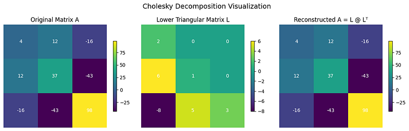Image 8: cholesky decomposition | image by author

Image 8 illustrates Cholesky Decomposition, a powerful technique in linear algebra. It starts with a Hermitian Positive Definite matrix**A**. Using Cholesky decomposition, we factorize A into a lower triangular matrix**L** such that equation 2 holds:

The last panel confirms this by showing that multiplying L by its transpose reconstructs the original matrix, as stated in equation 2.

To make computations more efficient, GPTQ uses this Cholesky decomposition. The Cholesky decomposition provides several benefits.

• Efficiency: It’s ~\(2\times\) faster than LU decomposition for solving linear systems.
• Stability: Helps maintain numerical stability in GPTQ quantization.
• Error Redistribution:In GPTQ, Cholesky is applied to the inverse Hessian matrix, allowing precise redistribution of quantization errors.

Algorithm#

Image 9: GPTQ algorithm from paper: https://arxiv.org/abs/2210.17323

Now lets go over the algorithm as mentioned in the paper:

1. Initialization:

• A zero matrix \(Q\) is initialized to store the quantized version of the weight matrix \(W\).
• A second zero matrix \(E\) is initialized to accumulate quantization errors for each block of columns.

1. Preprocessing:

• The inverse Hessian matrix H−1 is computed in advance, as given in equation 3

• To make computation more efficient, the Cholesky decomposition of this inverse Hessian is precomputed. This decomposition helps in scaling the updates during error compensation.

1. Block-wise Quantization:

• The algorithm processes the weight matrix W in blocks of columns of size B.
• For each column in a block:
• The column is quantized and the result is stored in the corresponding column of Q.
• The quantization error (difference between original and quantized column) is computed and scaled using the diagonal element of the Hessian inverse.
• This error is then propagated within the current block using the Hessian inverse to adjust subsequent columns.

2. Error Compensation for Remaining Weights:

• Once a block is processed, the accumulated error for that block is used to update all remaining weights to the right of the current block.
• This ensures that quantization-induced distortions don’t accumulate unchecked.

3. Efficiency and Accuracy:

• The algorithm proceeds from left to right across the matrix, quantizing and updating in blocks.
• This block-wise strategy ensures that local weight interactions are preserved and accounted for using second-order information, significantly improving quantization accuracy while keeping computational costs manageable.

If you are interested in the code, take a look at the quantize method in GPTQModel library.

Code#

Code 8

!pip install --upgrade -q accelerate optimum transformers
!pip install gptqmodel --no-build-isolation
!pip install -U "numpy<2" # GPTQ model does not work with numpy2

from transformers import AutoModelForCausalLM, AutoTokenizer, GPTQConfig
model_id = "meta-llama/Meta-Llama-3-8B-Instruct"
tokenizer = AutoTokenizer.from_pretrained(model_id)
gptq_config = GPTQConfig(bits=4, dataset="c4", tokenizer=tokenizer, model_seqlen=1024)
quantized_model = AutoModelForCausalLM.from_pretrained(model_id, device_map="auto", quantization_config=gptq_config)

Now lets quantize llama3 using GPTQ so that we can compare with earlier methods (Code 8). We can use the GPTQConfig class to directly quantize and load the model, but this was giving me memory error in colab.

Code 9

from gptqmodel import GPTQModel
model_id = 'astronomer/Llama-3-8B-Instruct-GPTQ-4-Bit'
model = GPTQModel.load(model_id)
tokenizer = model.tokenizer

So I loaded an already quantized model and used the GPTQModel class from the library (Code 9). Now we can get the gpu utilization and perplexity using our functions defined before. Below are the results.

Code 10

      Metrics    UnQ     Q  GPTQ
0      Memory  12.41  8.87  5.99
1    Time (m)  10.90  1.40  1.60
2  Perplexity   5.28  5.32  5.69

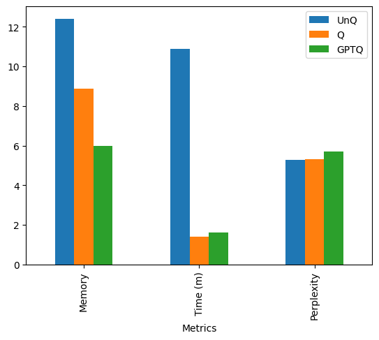Image 10: GPTQ: comparison with 8bit quantization

As you can see in Code 10, perplexity has gone down more: 5.69 compared to 5.32 as that of bitsandbytes. The memory has improved: 5.99 GB compared with 8.87 of bitsandbytes but the total time has degraded from 1.40 mins to 1.60 mins still far better than the unquantized model.

AWQ: Activation Aware Weight Quantization#

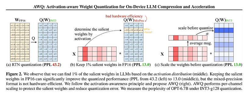Image 11: AWQ: Activation-aware Weight Quantization for On-Device LLM Compression and Acceleration

Moving on let’s talk about activation quantization or AWQ. It was published in June 1, 2023. Activation-aware quantization doesn’t quantize all the weights, but instead it preserves a small percentage of the weights that are important for LLM performance. This significantly reduces quantization loss such that you can run models in 4-bit precision without experiencing any performance degradation. So, let’s go over the theory a little bit.

If \(w\) is the weight matrix and \(x\) is the inputs, then the output activations \(y\) is going to be the matrix product of \(w\) and \(x\), as shown in equation 4.

If Q is both the quantization — dequantization weight matrix, then the goal is to find such a Q that the output of \(Q(w)x\) should be almost equal to \(y\) as shown in equation 5.

So we can bring in a scaling parameter \(\Delta\), in the absmax form, divide the weights by this \(\Delta\) and then perform a rounding operation on it. This will be the quantization operation. To perform the dequantization, we can multiply the quantized weights with the scaling \(\Delta\). This operation is shown in equations 6 and 7.

AWQ Quantization Error and Loss Function#

So now let’s explore the error Err due to quantization. We can define it as the absolute error between the actual output and the output due to quantization, giving equation 8. So, we can replace the \(Q(w)\) part with the formula that we had in the previous slide and divide the scale parameter \(\Delta\) to the actual weights w, giving equation 9 and equation 10. Thus, we can take out the \(\Delta\) from both the values, take it outside and also take out the inputs \(x\) from both the values and take it outside, arriving at equation 11. \(\Delta\) would be positive because if you see the formula for \(\Delta\), there is the absolute function there as well. The weights x would be positive because we will run them through the ReLU function which also keeps the value of \(\Delta\) only the positive values.

If we take the middle value and call it \(\text{RoundErr}(w/\Delta)\), as in equation 12, then we can replace the part with round error function, giving equation 13. We will use this later. If we assume each variable in \(W/\Delta\) is a uniform distribution, the absolute error will also form a uniform distribution in the range 0, 0.5. Expectation of the round error of \(W/\Delta\) is 0.25 which is constant, as in equation 14. In this case, the quantization absolute error of weight only quantization is proportional to the quantization scale \(\Delta\) and the input activation x. In a single group, \(\Delta\) is constant for everyone. So for a single group, this quantization error is proportional to x, as in equation 15. In other words, we can say that the quantization error of weight only quantization is activation aware. If the input activation magnitude is small, the quantization error is small and if the input activation magnitude is large, the quantization error is large. Therefore, if we could somehow reduce the input activation magnitude in weight only quantization, the quantization error can be reduced. These overall ideas are shown in equations 12–15.

So if we continue to the previous equations that we had discussed, equation 16, we want to reduce the magnitude of the activations in the input. We can inversely scale the activations and then to counter that, we will scale the weights as well, which is almost similar to quantizing the scaled weights as seen in equation 17 and equation 18. So now we can replace w by ws in the equations discussed in equation 19 and equation 20. Finally, we can give the error equation as seen in equation 21. If \(W/\Delta\) is a uniform distribution, then \(\text{RoundErr}(ws/\Delta')\) is also a uniform distribution and the expectation of that will also be 0.25, as shown in equation 22.

So now we can do a comparison between Err’ and Err, giving equation 23. We divide by both the forms because the expectation of the round error is the same. We cancel out the round error parts and also x gets cancelled. So the remaining becomes \(\Delta'\) by \(\Delta\) into 1/s, as shown in equation 24. We want to move towards lower error. That means Err’ needs to be less than Err. One way would be to go higher and higher s while keeping \(\Delta'\) close to \(\Delta\).

From the analysis till now, the objective can be said as finding the best s, per equation 25, where loss is the least squares between the difference between the quantized scaled weights and inverse scale of the activations and the original multiplication of the weights and activations, as defined in equation 26.

AutoAWQ Implementation#

Code 11

def quantize(self):
    for i in tqdm(range(len(self.modules)), desc="AWQ"):
        ...

        # [STEP 1]: Get layer, extract linear modules, extract input features
        named_linears = get_named_linears(self.modules[i])

        # Filter out the linear layers we don't want to exclude
        named_linears = exclude_layers_to_not_quantize(
            named_linears, self.modules_to_not_convert
        )

        input_feat = self._get_input_feat(self.modules[i], named_linears)
        clear_memory()

        # [STEP 2]: Compute and apply scale list
        module_config: List[Dict] = self.awq_model.get_layers_for_scaling(
            self.modules[i], input_feat, self.module_kwargs
        )
        scales_list = [
            self._search_best_scale(self.modules[i], **layer)
            for layer in module_config
        ]
        apply_scale(self.modules[i], scales_list, input_feat_dict=input_feat)
        scales_list = append_str_prefix(
            scales_list, get_op_name(self.model, self.modules[i]) + "."
        )

        # [STEP 3]: Compute and apply clipping list
        if self.apply_clip:
            clip_list = self._search_best_clip(
                self.modules[i], named_linears, input_feat
            )
            apply_clip(self.modules[i], clip_list)
            clip_list = append_str_prefix(
                clip_list, get_op_name(self.model, self.modules[i]) + "."
            )

        # [STEP 4]: Quantize weights
        if not self.export_compatible:
            self._apply_quant(self.modules[i], named_linears)

        clear_memory()

Now since we have gone through the theory, we can now go through Code 11 and it would make sense to us. The code is taken from casper-hansen/auto-awq. If you go through the quantize method, you will see step one is get the layer extract linear modules extract input features, and then we filter out the linear layers we don’t want to exclude. Then we search for the best scale and apply the best scale. Next, we compute the clipping list and apply the clipping list. Finally, we quantize the weights. The quantizing the weights is a part is simple. If we know the scales and the zeros, we can apply these scales and zeros and perform the quantization. So, point is how to search for the best scale. So, for this, we go to the search best scale method. Next, we can search for the best clip and apply that to the modules. Now that we have the quantized layers we can replace the original model with the quantized weights for the final model.

Code 12

def _compute_best_scale(
    self,
    x: torch.Tensor,
    w_mean: torch.Tensor,
    x_mean: torch.Tensor,
    module2inspect: torch.nn.Module,
    linears2scale: List[nn.Linear],
    fp16_output: torch.Tensor,
    kwargs: Dict={},
):
    """
    Compute loss and select best scales

    L(s) = || Q(W * s) (s^-1 * X) - W * X ||
    Q: weight quantization function | pseudo_quantize_tensor(W * s)
    X: inputs from calib dataset    | X
    W: original weights in FP16     | layer
    s: per channel scaling factor   | s^-1 * X
    """
    n_grid = 20
    history = []
    best_ratio = -1
    best_scales = None
    best_error = float("inf")

    org_sd = {k: v.cpu() for k, v in module2inspect.state_dict().items()}

    device = x.device
    x_mean = x_mean.view(-1).to(device)
    w_mean = w_mean.view(-1).to(device)

    for ratio in range(n_grid):
        # create new scales
        ratio = ratio / n_grid

        # NOTE: s^-1 * x is fused here, according to paper
        if self.duo_scaling:
            scales = (x_mean.pow(ratio) / (w_mean.pow(1 - ratio) + 1e-4)).clamp(min=1e-4)
        else:
            scales = x_mean.pow(ratio).clamp(min=1e-4).view(-1)
        scales = scales / (scales.max() * scales.min()).sqrt()
        scales_view = scales.view(1, -1).to(device)

        # avoid scaling values that overflow
        scales[torch.isinf(scales)] = 1
        scales[torch.isnan(scales)] = 1

        # Q(W * s)
        for fc in linears2scale:
            fc.weight.mul_(scales_view)
            fc.weight.data = (
                self.pseudo_quantize_tensor(fc.weight.data)[0] / scales_view
            )

        # W * X
        int_w_output = self._module_forward(x, module2inspect, kwargs)
        int_w_output = int_w_output.clip(torch.finfo(int_w_output.dtype).min,
torch.finfo(int_w_output.dtype).max)

        # compute mean squared error (L2 norm)
        loss = self._compute_loss(fp16_output, int_w_output, device)

        history.append(loss)
        if loss < best_error:
            best_error = loss
            best_ratio = ratio
            best_scales = scales.clone()
        module2inspect.load_state_dict(org_sd)

    if best_ratio == -1:
        logging.debug(history)
        raise Exception

    assert torch.isnan(best_scales).sum() == 0, best_scales

    return best_scales.detach().cpu()

Code 12 is the code related to computing the best scale. So for this, we start with the absmax of the weights. We compute the per-channel mean of the of the input activation with chunking. Then the weights * scale is pseudo quantized. Then we compute the output activation. Based on this activation the loss is calculated. So, we set the best scale based on wherever the loss is the minimum. Thus, you can see we are doing a grid search here. Next let's go to Code 13, the self._compute_loss function.

Code 13

def _compute_loss(
    self,
    fp16_output: torch.Tensor,
    int_w_output: torch.Tensor,
    device: torch.device,
):
    ...

    # Compute the loss for each chunk
    for fp16_chunk, int_w_chunk in zip(fp16_chunks, int_w_chunks):
        chunk_loss = (fp16_chunk.to(device) - int_w_chunk.to(device))\
            .float().pow(2).sum().item()
        loss += chunk_loss

    # Normalize the loss by the total number of elements
    loss /= num_elements

    return loss

In Code 13, the _compute_loss method, some chunking is done, but the important thing is the squared difference between fp16 chunk and the quantized w chunk is done and then they are summed up to get the chunk loss. The chunk loss are all added up and finally normalized by the total number of element to get the final loss.

Usage Code and Benchmarking#

Code 14

!pip install -q transformers accelerate autoawq

from awq import AutoAWQForCausalLM
from transformers import AutoTokenizer
model_id = "meta-llama/Meta-Llama-3-8B-Instruct"
quant_config = {"zero_point": True, "q_group_size": 128, "w_bit": 4, "version":"GEMM"}

# Load model
model = AutoAWQForCausalLM.from_pretrained(model_id)
tokenizer = AutoTokenizer.from_pretrained(model_id, trust_remote_code=True)

# Quantize
model.quantize(tokenizer, quant_config=quant_config)

Code 14 shows you can quantize using autoawq similar to how we had quantized before, by setting up a quant_config.

Code 15

      Metrics    UnQ     Q  GPTQ    AWQ
0      Memory  12.41  8.87  5.99  5.695
1    Time (m)  10.90  1.40  1.60  2.710
2  Perplexity   5.28  5.32  5.69  5.490

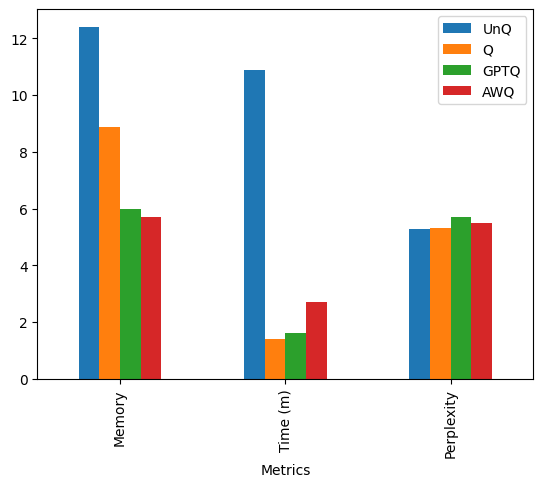Image 12: AWQ comparison

When compared with other models in Code 15, and especially GPTQ, the memory is the best till now, while total time for inference has degraded as compared with GPTQ. Interestingly perplexity is slightly better than GPTQ. As usual, make your own comparisons to find the best algorithm for your use case.

GGUF#

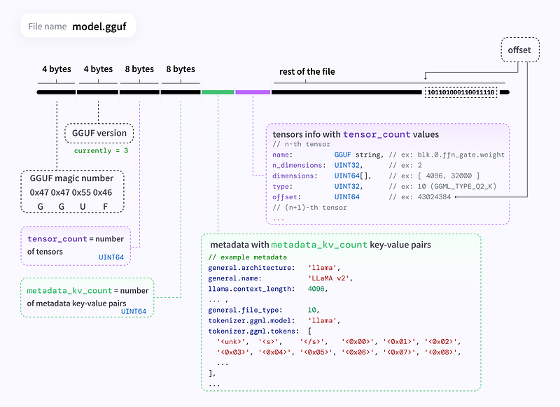Image 13: gguf file | source: GGUF

So now let’s talk about GGUF. GGUF was introduced by the llama.cpp team on August 2021–23. It’s a replacement for GGML. So GGUF is not a quantization technology but specifically it is used for storing the model weights and running them on consumer hardware such as our laptop or edge devices. Ideally any number of quantization techniques can be used in GGUF. Mostly you will find that they are weight quantization techniques with different hybrid schemes such int4 for some of the weights and int8 for some other weights. The specific quantization technique that is used is linear quantization.

GGUF Quantization Implementation#

The first four bits is the GGUF magic number then the next four bits is the GGUF version, the next eight bits is the tensor count and then the next eight bits is the metadata of the kv count. Then we have the key value pairs various metadata key value pairs and then the rest of the files with the tensor values so the quantization in GGUF is based on linear quantization. In linear quantization, we can take the quantization operation as the inverse scale of the weights w and a zero-point z and then we can do a rounding operation on that so the de-quantization process should remove the zero point and multiply with the scale now this scale can be the min max scale and scalar so we take the min max of x and the min max of the quantized range because we want to fit the full range of x to the full range of quantization, as in equation 27 and equation 28. So \(s = \frac{x_{max} - x_{min}}{q_{max} - q_{min}}\) as in equation 29, and hence \(z = q_{min} - \frac{x_{min}}{s}\) as in equation 30. The quantized value q is found using equation 31, and the dequantized value using equation 32.

The quant descriptions are mentioned in the hugging phase documentation. For example, Q4_1: 4-bit round-to-nearest quantization (q). Each block has 32 weights. Weight formula: w = q * block_scale + block_minimum. [source]

Code 16

class Q4_1(__Quant, qtype=GGMLQuantizationType.Q4_1):
    @classmethod
    def quantize_blocks(cls, blocks: np.ndarray) -> np.ndarray:
        n_blocks = blocks.shape[0]

        max = blocks.max(axis=-1, keepdims=True)
        min = blocks.min(axis=-1, keepdims=True)

        d = (max - min) / 15
        with np.errstate(divide="ignore"):
            id = np.where(d == 0, 0, 1 / d)
        qs = np.trunc((blocks - min) * id + np.float32(0.5), dtype=np.float32).astype(np.uint8).clip(0, 15)

        qs = qs.reshape((n_blocks, 2, cls.block_size // 2))
        qs = qs[..., 0, :] | (qs[..., 1, :] << np.uint8(4))

        d = d.astype(np.float16).view(np.uint8)
        m = min.astype(np.float16).view(np.uint8)

        return np.concatenate([d, m, qs], axis=-1)

So now if we go through the llama.cpp gguf code implementation in quants.py as shown in Code 16. Taking the same example of Q4_1 class, we have the max is the maximum of the block and minimum as the minimum of the block. So your denominator becomes a (max — min)/15. 15 because that is \(2^4 - 1\) where b=4 is the number of bytes. So then you can compute the quantization scale qs which is (max-min)/(range in the lower bit) as we have already discussed. Then you can apply the rounding function. This is how you calculate the quantized value. Check out the code in the source as well.

Code and Benchmarking#

Code 17

from huggingface_hub import hf_hub_download
model_id = "QuantFactory/Meta-Llama-3-8B-Instruct-GGUF"
filename = 'Meta-Llama-3-8B-Instruct.Q4_K_S.gguf'
model_path = hf_hub_download(model_id,
                             filename=filename,
                             local_dir='/content')
print("My model path: ", model_path)

I did not try to quantize the models because of high compute requirements and was only trying this out in colab, so downloaded the model from QuantFactory repo and saved in the content folder (Code 17).

Code 18

git clone https://github.com/ggml-org/llama.cpp
cd llama.cpp/
cmake -B build -DGGML_CUDA=ON
cmake --build build --config Release
./build/bin/llama-perplexity \
    -m /content/Meta-Llama-3-8B-Instruct.Q4_K_S.gguf \
    -f dataset.txt

Now we can install the llama-cpp-python and use the Llama class to get the results, but we need to calculate the perplexity. So we will use the perplexity command that is there in the llama.cpp repo and to do that we need to install llama.cpp from source. Then in the build folder we can access the llama-perplexity command, and we will pass the dataset. This will generate the perplexity for us (Code 18).

Code 19

      Metrics    UnQ  GPTQ    AWQ    GGUF
0      Memory  12.41  5.99  5.695  4.3620
1    Time (m)  10.90  1.60  2.710  1.4800
2  Perplexity   5.28  5.69  5.490  3.2154

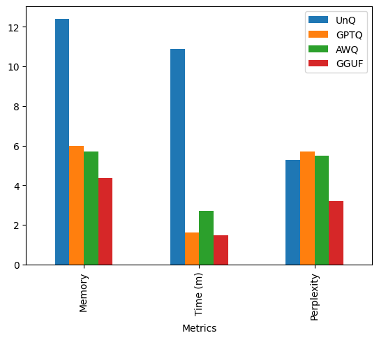Image 14: GGUF comparison

Now we can plot the comparison with GPTQ and AWQ from Code 19. You can see for the GGUF model, there is big improvement in all the metrics. Interestingly the perplexity is even better than the unquantized model which is slightly weird. Disclaimer here: Please don't deploy on my benchmarks, do your own checks before deploying to production.

HQQ: Half Quadratic Quantization#

Image 15: source: https://mobiusml.github.io/hqq_blog/

Now let's go over Half Quadratic Quantization. This came out in November 2023. In their blog they mentioned some points about previous quantization algorithms.

1. The calibration data that is used can negatively affect the quality of calibration.
2. Calibration can be a heavy computational process especially for large language models.

So in the blog they mentioned that they have developed this algorithm which minimizes errors in the weights themselves preserving the model’s fundamental building blocks. This method uses sparsity promoting loss function where we take lp norm<1 which more accurately represents the distribution of outlier weights which are often critical to model performance. They use mathematical decomposition to break the overall problem into simpler sub problems and solve those sub problems in a few steps instead of using gradient descent methods. They use closed form solutions for each step so that they can do things faster because gradient descent may take thousands of iterations. The quantization is done on the gpu with half precision and uses the CPU to transfer data once the solution is done.

HQQ Quantization Theory and Derivation of Algorithm#

Now lets go over the theory and try to derive the algorithm. This will give us an understanding of why the HQQ algorithm works like this and how to solves the previous problems. The notation is slightly different where Q means only quantization and \(Q^{-1}\) means dequantization. This is slightly different from what we had discussed in the AWQ section. So as seen in equation 33, the quantization is a function of zero-point z and scaling parameter s and we scale the weights W by s and then add the zero point and then perform rounding operation on it to get Wq, the quantized weights. Equation 34 shows the corresponding dequantization.

From this we can say that the dequantization operation is removing the zero point and then multiplying with the scale. If correct s and z are chosen, then post-dequantization the weights should be close to the original prequantization weights. So in equation 35, we can define the error of the weights due to the quantization dequantization process to be the difference between the original weights and the weights after the quantization dequantization process. If we define a monotonic function transformation \(\phi\) on this error E, we arrive at equation 36, which is defined as the arg min of the overall error condition on some specific z and s.

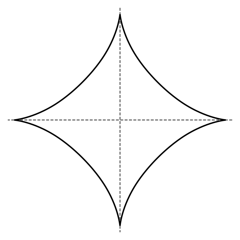Image 16: lp space, 0<p<1, source: Lp space — Wikipedia

In the paper the authors considered \(\phi\) as the lp norm of the error where p is between 0 and 1. They chose this because this is a sparsity promoting loss function. Defining \(\phi\) in this manner, as in equation 37, makes the equation nonconvex. In equation 37, i is there as a subscript of e denoting that the error considered is for the \(i^{th}\) block.

So, from equation 35, we can arrive at equation 39, where the quantization error is given by We, as defined in equation 38. After that they applied the penalty method where they applied \(\phi\) on this We and also applied a multiplying factor \(\beta\) on the difference between We and the quantization error for a specific z and We. The goal is to find the best z and We so that we reach the argmin of this augmented function. The authors assumed that scaling is assumed to be constant to make the equations and derivations simpler; so Q is only dependent on z. Notice that both the terms in equation 40 are positive, so we can optimize them independently. So we can find the minimum of the first term and then find the minimum of the second term and we will be able to arrive at the overall minimum.

Why this formulation in equation 39 works is because when \(\beta\) is large, this forces the solution of the We to be the same as the quantization error. And when \(\beta\) is infinite we recover the original problem exactly. But for finite \(\beta\), we have a smoother problem which we can solve iteratively.

Now lets say we are only trying to solve for the first term identified in equation 40, from the objective in equation 39, and only trying to solve for We. Let's denote that as u, the quantization error as x and denote the overall optimization equation as f(u) just to make it simpler to the eyes. So, \(f(u)\) is the sum of p norm of u and \((u-x)^2\) multiplied with \(\beta/2\), as in equation 41. This is just a rewriting of equation 39 with new terms, restricted to \(u > 0\) in equation 42. Since error will be positive, so can we remove the modulus operation here. We want to get to the minimum of this function f, so we can set derivative as 0, giving equation 43, and then rearrange some terms, giving equation 44 and equation 45. This results in the final equation for u.

Now lets look at equation 49. Since \(p\) is between 0 and 1 and \(\beta\) is large, we can absorb \(p\) in \(\beta\), giving equation 46. So \(p/\beta\) is just written as \(1/\beta\). Since \(u\) must be positive as its just another term for We, so we can write that the minimum value of \(u\) will be 0 and hence this is given by \(\max\left(0, x - \frac{1}{\beta}u^{p-1}\right)\), as in equation 46. In equation 47, since we want the best We aka \(u\) to be the same as quantization error \(x\), hence we replace \(u\) by \(x\). This means that when we apply the shrinking operation, as in equation 48, this is the same as multiplying with the \(\operatorname{sign}(x)\) function and the function \(|x| - \frac{|x|^{p-1}}{\beta}\) clipped at 0. Hence this can be the We at for the next iteration t+1, giving equation 49, and we change the max function clipped a 0 with the relu function which is mathematically equivalent by definition.

So, we can see that the 1st term in equation 40 is reduced, giving equation 50, so we can take a look at the 2nd term of the equation. We have found the best \(W_e\) for the next iteration (t+1), so we will replace We with \(W_e^{t+1}\) and say that now we only need to optimize for \(z\), as in equation 51. Equation 52 tells us that the new quantized weights \(W_q\) is the inverse scaling of \(W\), and we add the current \(z\) and then we perform the rounding operation. So the dequantized version, shown in equation 53, would be scaling \(W_q^{t+1}\) with s and then removing the \(z\). We can now use this definition of \(Q^{-1}\) and replace the \(Q^{-1}(Q(W))\) part of the equation, arriving at equation 54.

So now we can take the equation for t2 in equation 54, giving equation 55, and remove all the brackets, giving equation 56. In equation 57, we can bring \(-z\) to the front, \(sW_q^{t+1}\) term after that, then \(-W\) and then \(W_e^{t+1}\). In equation 58, inverting all the signs because doing that has no effect on \(l_2\) norm (Homework: check the validity of this statement). In equation 59, we again do some bracketing. In equation 60, we take the s outside the bracket.

We have now arrived at the equation for the t2 term, equation 61. This has the same form of \(\min \lVert z-a \rVert^2\), as in equation 62. Analytically, the solution where the norm is the minimum is when \(z = a\), per equation 63 (do you see it?). So, we can say that reducing t2 means, in step (t+1) the value of z we can consider to be \(W_q^{t+1} - \frac{W - W_e^{t+1}}{s}\), as in equation 64. I am not sure where the s went but this is the term that the solution that they mentioned in the paper and the blog.

Quantization is done in a block or similar group. This means that z is shared across the group solution and becomes the mean over the relevant data set. This last line, equation 65, means that we are taking the mean in the group for the next value of z.

HQQ Algorithm and Implementation#

Now having discussed all this theory, we can talk about the final algorithm. In the first step we find the next value for \(W_e\). This comes from equation 66. Once we have the best value for \(W_e\) for the current z, we find the best value for z which comes from equation 67. Finally, we increase \(\beta\) by some constant \(\kappa\), as in equation 68, so that beta keeps on increasing in each iteration. This was one of the initial conditions when specifying the penalty method in equation 39, and based on which all the derivation lies.

Code 20

def optimize_weights_proximal_v2(
    ...
    # Optimize for zero-point
    best_error = torch.tensor(1e4, dtype=torch.float32, device=device)
    scale_prev, zero_prev = scale.clone(), zero.clone()
    for i in range(iters):
        W_q = torch.round(W_f * scale + zero).clamp(min_max[0], min_max[1])
        W_r = (W_q - zero) / scale

        # current_error = float(torch.pow(torch.abs(W_f - W_r), max(0.80, lp_norm)).mean())
        current_error = torch.abs(W_f - W_r).mean().float()

        if verbose:
            print(i, np.round(current_error, 6))

        if early_stop:
            if best_error - current_error > tol:
                best_error = current_error
                scale_prev, zero_prev = scale.clone(), zero.clone()
            else:
                scale, zero = scale_prev.clone(), zero_prev.clone()
                break

        W_e = shrink_lp_op(W_f - W_r, beta, lp_norm)
        zero = torch.mean(W_q - (W_f - W_e) * scale, axis=axis, keepdim=True)
        beta *= kappa

If you see in Code 20, the official implementation of HQQ, this algorithm is implemented. Each iteration we compute the quantized weights W_q and the de-quantized weights W_rfor the best zero found in the last iteration. So, we find W_e based on the shrinking_lp_op and then we find the zero which is the mean of (W_q — (W_f — W_e)*scale) as per the formula. Then we increment beta with kappa. They took inverse scale instead of the scale because it they found that it helps better with stability of the algorithm. That is why there is a multiplication with scale instead of doing divide by scale as mentioned in the theory. Also note in the code that, if the error is not improving it means that we have found the minimum and then we come out of the loop. This is the early stop condition.

Code 21

def shrink_lp_op(x: Tensor, beta: float, lp_norm: float) -> Tensor:
    ...
    out = torch.abs(x)
    out.sub_((1.0 / beta) * out.pow(lp_norm - 1)).clamp_min_(0.0)
    out.mul_(torch.sign(x))
    return out

In Code 21, the shrinking operator function shrink_lp_op, first the absolute value is taken, then we raise to the power of (lp_norm-1) and then multiply with 1/beta and then we do clamp minimum instead of taking the relu function. And then we multiply with the sign function. This is in line with the resolution for \(W_e^{t+1}\) with some coding modifications, that I am assuming, for the sake of making the code faster.

Code and Benchmarking#

Code 22

!pip install -q hqq

import torch
from transformers import AutoModelForCausalLM, AutoTokenizer, HqqConfig
quant_config = HqqConfig(nbits=4, group_size=64)
model_id = "meta-llama/Meta-Llama-3-8B-Instruct"
tokenizer = AutoTokenizer.from_pretrained(model_id)
model = AutoModelForCausalLM.from_pretrained(
    model_id,
    torch_dtype=torch.float16,
    device_map="cuda",
    quantization_config=quant_config)
model = torch.compile(model)

# benchmarking
get_gpu_memory_utilisation()
calculate_perplexity(model, tokenizer, dataset, model_id)

Code 22 shows running HQQ quantization, done using the general huggingface pattern where we create the config and pass the config to AutoModelForCausalLM. We can choose different configuration such as nbits and group_size. Based on this we can do the benchmarking.

Code 23

      Metrics    UnQ    AWQ    GGUF     HQQ
0      Memory  12.41  5.695  4.3620  6.0330
1    Time (m)  10.90  2.710  1.4800  3.9000
2  Perplexity   5.28  5.490  3.2154  5.5294

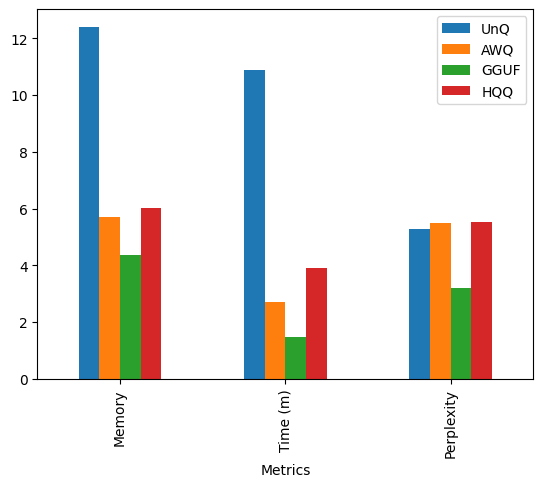Image 17: HQQ Comparison

In my experiments in Code 23, HQQ is slightly higher than AWQ and if you remember AWQ was activation quantization while HQQ is only weights. You might be disheartened to see that after so much high level maths the results are quite poor but don’t discount HQQ so fast, the algorithm is really quite fast. It is probably the only one that I could complete in colab, for the other models I had to download already quantized models so in a way this is quite good. Maybe in your case you might actually get good results so try it out and reach out to me and we can discuss more on this. I have shared my linkedin link at the end.

BitNet#

Till now we have been talking about 8-bit and 4-bit quantization techniques. Currently 4-bit quantization with some amount of Qlora training is the industry standard. The next frontier in this field is somewhere between 1-bit and 2-bit LLMs. The most famous of these models is the bitnet by Microsoft. Checkout the history of bitnet implementation. I will write the ones which I think are the major milestones.

• 10/17/2023 BitNet: Scaling 1-bit Transformers for Large Language Models. Here they experimented with pure 1 bit.
• 02/27/2024 The Era of 1-bit LLMs: All Large Language Models are in 1.58 Bits. But then they found that just 1 bit is not making the cut. So they moved to 1.58 bits.
• 10/17/2024 bitnet.cpp 1.0 released.
• 10/21/2024 1-bit AI Infra: Part 1.1, Fast and Lossless BitNet b1.58 Inference on CPUs. This is about how to efficiently store in the hardware using efficient bitpacking algorithms.
• 11/08/2024 BitNet a4.8: 4-bit Activations for 1-bit LLMs. This is the current final architecture.

1.58 bits?#

Image 18: A cat can alternate between solid liquid and gas | source https://shirtoid.com/204331/three-states-of-matter/

Lets first understand the rational behind the name 1.58. Our current hardware system is made up of bits. It means you have two values in your representation. If you want to store 4 values, you need 2bits. 10-bit means you have 2 to the power 10 values. So, if you have 3 values that means 1-bit is not enough while 2-bits is too much. So in bit system you need \(\log_2(3) = 1.58\) bits. Or if your hardware can support 3 values in a single bit (also called a trit) then you need \(\log_3(3) = 1\) trit. Make sure that this logic makes sense before we proceed.

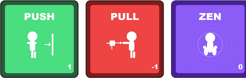Image 19: showcasing 1, -1 and 0 with push, pull and zen

You can choose any 3 numbers as the values in your ternary number system. In traditional matrix multiplication, you have many floating point operations. But notice that in this new system if you have the numbers plus 1, 0 and minus 1 that means selecting the value if it is plus 1, not selecting the value if it is 0 and penalizing the value if it is minus 1. As per experiments in the paper, this can result in 16 times faster operations.

Quantization Formula#

Equation 69 is for weight quantization to -1, 0 and 1. Equation 70 and equation 71 are for activation quantization based on the quantization type, whether int4 quantization is done or int8 quantization is done. Here \(\alpha\), \(\beta\) and \(\gamma\) and the mean of the absolute values of the block, mean of the absolute values of the activations and the max of the activation values in the block. \(\epsilon\) is a small value so that we dont have rounding error.

Architecture#

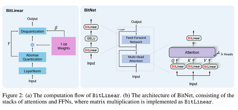Image 20: source: 2310.11453

Image 20 showcases that the Q, K, V, and Out projection as well as the Feed-forward networks are changed to BitLinear layers.

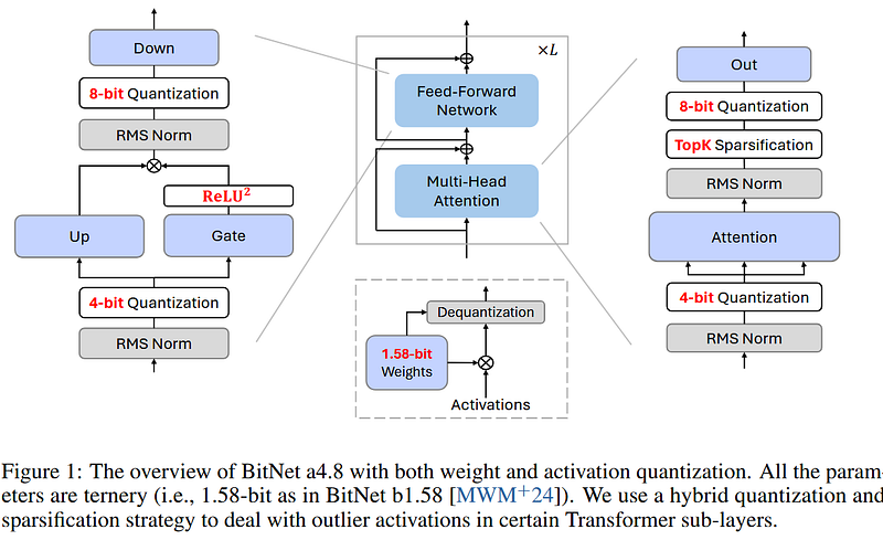Image 21: source: https://arxiv.org/pdf/2411.04965

Regarding the activation quantization, as mentioned in the previous section a mixture of 4bit and 8bit quantization is used. Notice that the input activations are generally in 4-bit quantization while the output activations are generally maintained at 8-bit activations in the layer. Another interesting change in the paper, they did 50% top-k sparsification for the attention scores. This strategy along with hybrid quantization is done to reduce the errors due to outlier channels of the activations. Also, there is the benefit of reducing the computational requirements of the model.

Another reason why Bitnet is fast and takes up less memory is because of the use of efficient storage technique also known as bitpacking. The authors compared between two strategies TL2 and TL1. LUT (Look Up Table) based algorithm is used to efficiently calculated the outputs. So quantization is not the only reason that BitNet is fast, there are a lot of other improvements also go in to make inference faster.

Code 24

!bash -c "$(wget -O - https://apt.llvm.org/llvm.sh)"
!git clone --recursive https://github.com/microsoft/BitNet.git
%cd BitNet
# Pip installation
!pip install --upgrade pip  >> log.bitnet
!pip install -r requirements.txt >> log.bitnet
# download the model and convert
hf_model_name = "HF1BitLLM/Llama3-8B-1.58-100B-tokens"
model_quant_type = "tl2" # tl1 or tl2
!python3 setup_env.py --hf-repo {hf_model_name} -q {model_quant_type}  >> log.bitnet
# run perplexity
!./build/bin/llama-perplexity -m models/Llama3-8B-1.58-100B-tokens/ggml-model-tl2.gguf -f dataset.txt

Code 24 shows how to run bitnet: we need to do some LLVM installs and then install bitnet from scratch. Bitnet.cpp code is formed from llamacpp. Hence running process is quite similar to GGUF as we have seen earlier. Similarly, we can also calculate the perplexity using the llama-perplexity command. But the perplexity that we are seeing is quite low. Now you might be wondering why we discussed on this topic if its not that usable as compared to other algorithms that we have discussed till now. I believe we are almost there with BitNet and things will be comparable soon.

Finally, we are at the end of this blog. Thanks for reading this lengthy article. I tried to give a comprehensive and non trivial view into the various popular algorithms related to LLM Quantization such as GPTQ, AWQ, GGUF, HQQ and BitNet. Special thanks to Abhishek Kumar, a lot of the content in this post is based on our discussions. If you want to discuss about your project or career please reach out to me at LinkedIn or Topmate.

References:#

• Colab notebook: https://colab.research.google.com/drive/1p5TVl_I5dFf3K2njZ76EXuPxcUtpI0ZU
• Perplexity — Wikipedia
• GitHub — huggingface/optimum-quanto: A pytorch quantization backend for optimum
• LLM int8 paper: https://arxiv.org/abs/2208.07339
• GPTQ paper: https://arxiv.org/abs/2210.17323
• Hessian matrix — Wikipedia
• Cholesky decomposition — Wikipedia
• AWQ: Activation-aware Weight Quantization for On-Device LLM Compression and Acceleration
• Auto-AWQ: AutoAWQ/awq/quantize/quantizer.py at main · casper-hansen/AutoAWQ · GitHub
• GGUF quantization: https://huggingface.co/docs/hub/en/gguf#quantization-types
• Penalty Method: Penalty method — Wikipedia
• BitNet history: https://github.com/microsoft/BitNet?tab=readme-ov-file#whats-new
• Ternary Number System: https://en.wikipedia.org/wiki/Ternary_numeral_system