The MATH behind Diffusion Models—DDPM

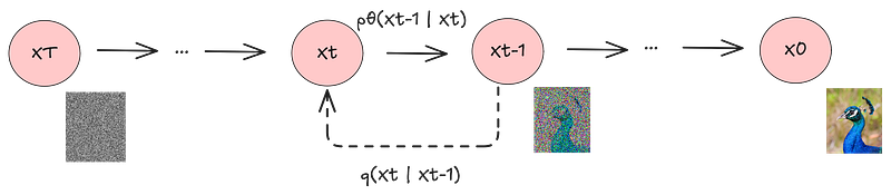
Graphical model as in the DDPM paper

The goal of AI is to learn from data, adapt to new and complex situations and solve problems without the need for human interventions.

This generally involves some form of intelligent signal generation that cannot be done with the help of some clean mathematical formula. To achieve this signal generation in complicated environments, generative models are used. Currently there are two classes of generative models that are quite successful: Autoregressive models and Diffusion models.

Diffusion models are widely used for various purposes such as

• Image generation from scratch using a prompt
• Inpainting and Conditional Image Generation
• Audio and Music Generation
• Video Generation
• Drug Discovery
• Training robots for household chores

And many more...

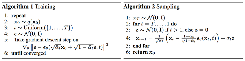source: https://arxiv.org/abs/2006.11239

In this blog we will take a look at how the diffusion process is formulated in the DDPM paper and how the training and sampling algorithms are formulated. The algorithms are shown in the screenshot above.

Watch on YouTube

Do also take a look at the video above for great visualizations on the topic.

Background and Motivation#

source: Pin by Carol📸 on Pixel art😻 in 2025 | Pixel art pattern, Easy pixel art, Pixel art

Now understanding what diffusion is, lets backtrack a little bit and we will consider the image example as that is both the easiest and where diffusion models first came into prominence.

An image is generally stored as a combination of red, blue and green pixels because our eyes have cones for these three colors and in this way, we are able to differentiate between a wide range of colors [source]. So, there are 3 channels for the pixels, and each channel has intensity values from 0–255 for the corresponding colors. So, the dimensions of the image are 1xCxHxW where C is the channels, H and W are the height and width of the image.

Now consider a random combination of these pixel values. It will probably be just some random noise image and not have anything discernible in the image. So, you can imagine that a “good” image would be just a very small subset of the overall class of images that can be denoted by this hyperspace denoted by 1xCxHxW. If we can somehow find the boundaries of this subspace, then maybe we will be able to generate an image out of this. GANs work on this idea where the Discriminator differentiates between the “real” and “fake” images and then conditions the Generator model to generate or sample from this subspace where the “real” reside. Another popular idea has been using Variational Autoencoders where the model learns a structured and continuous latent space and this is used to generate new data. Interestingly there have been major issues with these two approaches such as mode collapse in case of GANs and noisy images in case of VAEs.

Physical Diffusion#

Machine learning has had a history of taking inspiration from nature and this time we can take inspiration from diffusion process. You might have observed that when you dissolve one liquid like let's say some form of a die, it tends to distribute over the liquid. Thus, diffusion is the net movement of a body of molecules from a place of higher concentration to lower concentration within the domain of fluids. Although called diffusion, what we are more interested in is Brownian motion which is diffusion of a single particle. The reason for this will be clear later in this blog.

There is a poem from 60 BC which talks about the random movement of dust. The discovery of Brownian motion is attributed to botanist Robert Brown who observed the jittery behavior of pollens when working on an experiment. He first thought that pollens had life of their own but then experimented with inorganic matter as well confirming that this is not the reason. Albert Einstein proved the relation between the probability distribution of Brownian motion and the diffusion equation. The first complete and rigorous mathematical analysis of Brownian motion was given by Norbert Weiner and hence the Brownian motion is also called the Weiner process.

Markov chain Monte Carlo and Langevin Dynamics#

Since we are working on creating a generative model, we want to find the distribution of the true images. But notice carefully, we only want the true distribution to be able to sample from it. If finding the true distribution is hard, maybe another method can be used which is easier and which lets such somehow sample from the true distribution and thus, circumvent the whole problem.

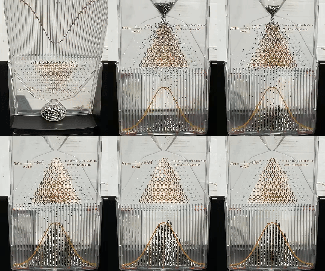source: https://www.youtube.com/shorts/MnBBV73KbDo

Markov Chain Monte Carlo (MCMC) is a class of algorithms that lets us do just that. Given a target and unknown probability distribution, one can construct a Markov chain which can be used to approximate this target probability distribution. The more steps that are included to perform the approximation, the more closely the distribution of the sample will match the true distribution. Notice that the idea is quite similar to the penalty method that we discussed in the previous blog. A process is Markovian when the current decision only depends on where you are at and not where you started. There is a probability transition matrix, and we can build a chain structure which is called a Markov chain.

Langevin dynamics is done of the most popular MCMC methods out there. If we have a probability distribution p(x) that is Markovian, then it will belong to the exponential class of distributions. This is given in equation 1 where f(x) is some function such that the equation holds. Let’s assume that we don’t have a way to directly sample from this distribution. Let’s assume that we can only know the gradient of the function at every point ∇f(x). If that’s the case we can apply gradient descent to find the modes of the distribution. This is given by equation 2 where η is the learning rate at time step t. If we can find the modes of the distribution, then we can find the areas with peaks in the density. Since in our training data, there will be lots of “good” images, this means going to peaks will result in these good images. Langevin sampling is an interesting modification of this gradient descent algorithm given by equation 3. Here we are adding a noise term to each step in the GD formula.

One problem can be that if want to speed up the process we might choose the value of \(\epsilon\) to be too high which may make the above equation 3 unstable and diverge out. So, it would be good if we can provide some form of guarantee that the update rule will converge. For this we can take the help of various algorithms such as the Metropolis Hastings algorithm. Not going into them as that is not the focus of this post.

Forward Diffusion#

Graphical model as in the DDPM paper

So, taking inspiration from this concept about Markov chains, lets say we sample an initial data \(x_0 \sim q(x)\) from a real data distribution. We gradually add noise to this initial data \(x_0\) similar to the physical diffusion we discussed above.

In this way we obtain a series of noisy data \(x_1, \dots, x_T\). Since a Markov process is memoryless, we can represent the joint probability of all data by equation 4 above. This is called the forward diffusion in DDPM paper.

Recall that a normal distribution is defined by a mean \(\mu\) and a variance \(\sigma^2 \ge 0\). Hence this transition kernel \(q(x_t \mid x_{t-1})\) is defined by a normal probability distribution with mean \(\sqrt{1-\beta_t}\, x_{t-1}\) and variance \(\beta_t I\). Here \(\beta\) is a noise variance schedule that exists in each iteration from \(\beta_0\) to \(\beta_t\) where \(\beta\) lies between 0 and 1, \(\beta \in (0, 1)\). \(I\) is the identity matrix.

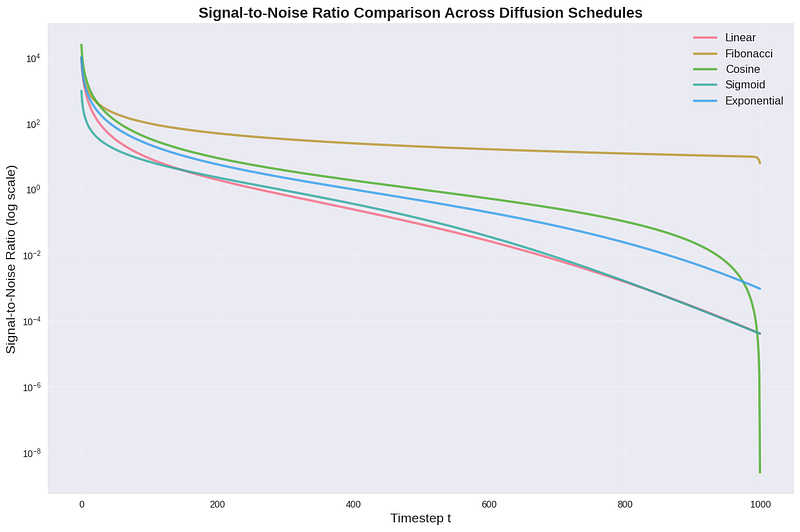
As mentioned \(\beta\) for a specific time t is given by a variance schedule \(0 < \beta_1 < \beta_2 < \dots < \beta_T < 1\). The specific way this can be changed can be according to various strategies such as linear, fibonacci, cosine, sigmoid, exponential and so on. The comparisons of the various decays of signal to noise ratio is shown in the above figure. The original DDPM paper used a linear schedule increasing from \(\beta_1 = 10^{-4}\) to \(\beta_T = 0.02\) but later works showed that using a cosine schedule is better. Since we are talking about the multidimensional scenario hence the equation has the identity matrix I, indicating that we are having the same variance \(\beta_t\) for all the dimensions.

Tractable Closed for Sampling at every step: Reparametrizing trick#

Now one challenge is if we want to sample x for the t=500 or more, do we need to repeatedly apply q 500 times? You may say that lets do dynamic programming (DP), but what if we don't want to do training sequentially!

There is in fact a better method available. Since we are using Gaussian distributions is a reparameterization trick which can help us find a tractable closed form sample of xt at any step.

If there is a normal distribution with mean \(\mu\) and standard deviation \(\sigma^2\), then this can be reparametrized to a linear form of \(\mu\), \(\sigma\) and a normal distribution with mean 0 and standard deviation 1. For \(x_t\) we can replace the mean and standard deviation terms from equation 5 to arrive at equation 6 above.

Now we take the same equation 6 in the first line. If we consider \(\alpha = 1 - \beta\) as in equation 7, then we can write \(x_t = \sqrt{\alpha_t}\, x_{t-1} + \sqrt{1-\alpha_t}\, \epsilon_{t-1}\) given by equation 8. Now we can apply the same reparameterization trick again to go from \(x_{t-1}\) to \(x_{t-2}\) in equation 9. If we now remove the brackets, we get an equation of three terms involving \(x_{t-2}\), \(\epsilon_{t-2}\) and \(\epsilon_{t-1}\) as shown in equation 10. We have 3 variables now and it would be simpler to go to 2 variables. Is there a way we can combine the \(\epsilon_{t-2}\) and \(\epsilon_{t-1}\) to a single term of \(\epsilon_{t-2}\)!

First two lines, equation 11 and 12, mean that we can consider the \(\epsilon_{t-2}\) and \(\epsilon_{t-1}\) terms as normal distribution with mean 0 and respective variances. From the laws of statistics, if we want to combine two normal distributions X and Y to Z, that means the new distribution is also a normal distribution with sum of the mean and the variances in equation 13. Sums are 0 so no need to worry about it. For the sum of variances in equation 14, we combine the terms, then resolve the brackets. \(+\alpha_t\) and \(-\alpha_t\) gets canceled. Finally, we get the form in equation 15 which is \(1 - \alpha_t \alpha_{t-1}\). In equation 16, we can combine the normal equations in 11 and 12 in the form of \(\epsilon_{t-2}\). We bring in a square root over the variance part.

Now taking equation 10 derived earlier, which consists of terms \(x_{t-2}\), \(\epsilon_{t-2}\) and \(\epsilon_{t-1}\), and using equation 16 where we reparametrized two normal distributions, we get the terms involving \(x_{t-2}\) and \(\epsilon_{t-2}\) such that the term under the square root is in a nice form of the manner \(\alpha_t \alpha_{t-1}\) as shown in equation 17. We can now extend this concept recursively till \(x_0\) which means that the term under the square root also keeps extending till \(\alpha_1\) as shown in equation 18.

So, in equation 19, we can write the whole term as the product of all the \(\alpha\)'s for all the time steps. If we write this product as \(\bar{\alpha}_t\), then we arrive at equation 20 where \(\bar{\alpha}_t = \alpha_1 \times \alpha_2 \times \dots \times \alpha_T\). This we can write as taking sample from a normal distribution with mean \(\sqrt{\bar{\alpha}_t}\, x_0\) and variance \((1 - \bar{\alpha}_t) I\), where \(I\) is the identity matrix.

Thus, we will not need to sample from q again and again and this makes the process much faster.

Reverse Diffusion#

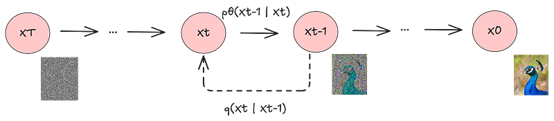Reverse diffusion here means going from left to right

But the forward diffusion by itself is not very useful. What would be interesting is doing the exact opposite i.e. transforming a totally random noise into an actual image. As per eq (5), the current value of x i.e. \(x_t\) is dependent on both the current value of \(\beta\) given by \(\beta_t\) and the previous value of x given by \(x_{t-1}\), so you can see that starting from \(x_0\) there will be a sequence of x's i.e \(x_1, x_2, \dots, x_T\), where \(x_T\) is pure Gaussian if the noise scheduling is done properly.

Now lets assume that there is a conditional probability \(p(x_{t-1}| x_t)\) which is the opposite of the forward diffusion process. If we could somehow compute this conditional probability for the reverse process, we could start from some random Gaussian noise \(x_T\), and then repeatedly “denoise” it so that we arrive at a sample from the real distribution \(x_0\). However, practically speaking, computing this probability distribution p will be quite difficult. In the paper they say its intractable because it means you need to consider all possible images in order to compute this conditional distribution. You can argue that in statistics in any case, we make do with sample statistic instead of the population statistic assuming that the law of large numbers will hold. Even then computing the probability distribution would be quite difficult if we do not make any assumptions about the distribution.

Two things are done that makes our lives easier. One is that we use a neural network to approximate this probability distribution. So we are learning \(p_\theta(\)x_{t-1} | xt)$, where \(\theta\) is the parameters of the neural network, which we will update during the training process.

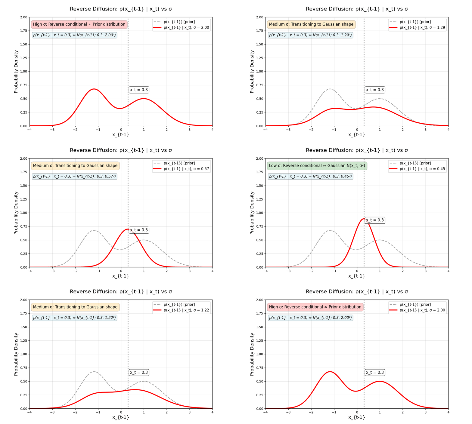reverse diffusion is gaussian!

Second interesting insight is that learning to reverse each intermediate step may be easier than learning to sample from the target distribution in one step. Taking inspiration from Weiner processes and Brian Anderson, 1982 it can be shown that this reverse conditional distribution \(p(x_{t-1}|x_t) \sim N\) is the forward process is Gaussian and the noise that is introduced is small. Basically “with sufficiently small step sizes” the authors in the DDPM paper said that the discrete diffusion process approaches the solution to a stochastic differential equation (aka Weiner Process / Brownian Motion) as the step sizes get infinitesimally small. Similar to how a binomial distribution approaches a normal distribution as n goes to infinity, so people will just approximate binomial as a Gaussian.

We can parameterize the reverse process in terms of \(\mu_\theta\) and \(\Sigma_\theta\) where the mean and the variance is a function of the noise level at time t as given in equation 22. We will come back with a derivation for this later.

Similar to the forward process in equation 4, we can write the joint distribution of all the images as the product of the individual models for the time steps as shown in equation 23 above. If we are able to compute the Gaussian parameters \(\mu_\theta\) and \(\Sigma_\theta\) mentioned in equation 22, we will then be able to compute for this joint product in equation 23 for all the time steps.

Above equation 24 simply means that the final image \(x_T\) is pure Gaussian noise with mean 0 and variance 1 in all dimensions. This is what we want to achieve after \(T\) steps in the forward diffusion, and what is our starting point in case of reverse diffusion.

Evidence Lower Bound Method#

Now lets assume that there is a latent variable \(z\) which is generating out data, which then becomes the joint probability \(p(x, z)\). Generally, in machine learning, we learn a model to maximize the likelihood of \(p(x)\) given all observed values of \(x\).

To compute this \(p(x)\) we can try to integrate over the whole of \(z\) as given in equation 25.

Another way of computing the \(p(x)\) is by utilizing the law of conditional probability, which makes it the ration of the joint probability \(p(x, z)\) and the conditional probability \(p(z|x)\). But both these formulations are not exactly great because equation 26 means that we will need to integrate over all the latent variables z or we need a ground truth model for the latent variable \(p(z|x)\). Here we know the numerator part because we have the data.

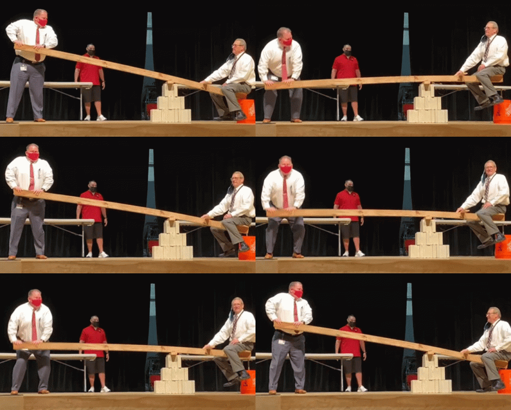Using a lever | Source: https://tenor.com/view/fulcrum-lever-gif-22681762

Now in case you are wondering if these equations are so useless, why did I talk about them in the first place. It turns out that using these two equations, we can derive a term called the Evidence Lower Bound (ELBO)which suggests a way to specify a lower bound on the evidence. The evidence in this case is the log likelihood of the observed data. This is equivalent to using a lever where it is difficult to lift the original object.

Now assuming we are training a model \(q_\phi(z|x)\) to approximate the true distribution \(p(z|x)\). This means that the joint distribution \(q_\phi(z, x)\) is the product of the conditional probability \(q_\phi(z|x)\) and \(q_\phi(x)\) as per the definition of conditional probability, shown in equation 27. In equation 28, we can know from the laws of probability, that the prior probability \(q_\phi(x)\) can be achieved by integrating over the whole joint distribution \(q_\phi(z|x)\) if we integrate over \(z\). So in equation 29, we can expand \(q_\phi(z, x)\) to the product as give in equation 27.

If we observe equation 29, from the perspective of z, \(q_\phi(x)\) is basically a constant, so we can take that outside the integration as shown in equation 30. Next we should be able to cancel out the \(q_\phi(x)\) in equation 30 because probability lies between 0 and 1 i.e its a positive number. Hence we get the relation in 31. We can also write the integration of \(q_\phi(z|x)\) over z as 1 because no matter what the evidence x is, something will happen to z.

From equation 31 we can multiply \(\log p(x)\) on both sides to arrive at equation 32. Then we can take the \(\log p(x)\) inside the integration sign for equation 33. Considering \(\log p(x)\) as the random variable, this can be rewritten in terms of statistical expectation as given in equation 34.

See above in equation 26, the joint probability can be written as a ratio or probabilities, and we can replace the \(\log p(x)\) as the same ratio in equation 35. Then we introduce \(q_\phi(z|x)\) in both the numerator and denominator in equation 36.

Let's take a slight detour and go through the derivations of one of the classic results in statistics. You might already know about this result, so consider this a refresher. The first line shown in equation 37, is the definition of the joint expectation when we add two random variables. In the next line with equation 38, we can separate out the summation terms and also interchange the x summation and y summation for the second term. In the third line with equation 39, we take out the x variable from the y summation and y variable from the x summation. This means in the fourth line in equation 40, the x join distribution is redundant and for the second term the y joint distribution is redundant, and we can thus write the probability in y and x terms respectively. This gives us the result in equation 41 which means that the sum of the expectation is the expectation of the sum. We will use this result shortly.

Now going back to equation 36, we write the same equation above in the first line. Since log of the product is the sum of the logs (log (AB) = log A + log B), we can separate out the product with an addition of two terms; the first term is ratio of joint probability p(x,z) and the model $q_\phi(z|x); the second term is the ration of model $q_\phi(z|x) and the conditional probability p(z|x) as shown in equation 42. Using the relation that we had derived in equation 41 that expectation of the sum is the sum of the expectations, we separate out the expectations in equation 43.

Thus we arrive at equation 44, where we can observe that the second term is the KL divergence between the approximate posterior $q_\phi(z|x) and the true posterior p(z|x). Since KL divergence will always be some positive value or at best be 0, we can say that log p(x) is lower bounded by the ELBO term given in equation 45.

Applying the ELBO method#

Because we started with saying that the forward process is Markovian as mentioned in equation 4 and 5, hence we can bring in an extra conditioning term x0 that is earlier in the chain, and this will not change the probability as shown in equation 46. Now applying Bayes rule to convert this to the ratio as shown in equation 47.

Now we will do the same ELBO analysis as shown in equation 45 and work towards maximizing the log of the evidence. Hence \(log p(x)\) is the log of the overall integration for \(p(x)\) for all the time steps as shown in equation 48. We can divide with same conditional probability \(q(x_{1:T}|x_0)\) in both numerator and denominator and this will not change the result shown in equation 49. This looks like the log of the expectation of p/q over all the time steps as shown in equation 50. Hence, we can utilize the ELBO relation we found in equation 45, where we can take the expectation outside and the log inside, to say that this will be greater than the expectation of the log of the ration of p/q.

As a result from equation 51, our ELBO part becomes the expectation from time step 1 to T which is the log of the ration between reverse diffusion probability and the reverse diffusion probability as shown in equation 52.

In the numerator we can replace the reverse diffusion with the product of the final noisy image at time step \(T\) and the conditional probability of the previous step given the current step taking from equation 23.

For the denominator, using equation 4, we can write the forward diffusion in terms of the product of the conditional distributions as in equation 54. We can add the \(x_0\) as a condition based on the arguments related to equation 46. Finally in equation 55, the ELBO part can be written as the expectation of the log of the probability of the final image at time step T, the conditional probability of the first image given the second image \(p(x_0 \mid x_1)\) and the product of the intermediate conditional probabilities in the reverse direction assuming parameters are \(\theta\). Notice that we extracted out the model at the first time step \(p_\theta(x_0 \mid x_1)\) so the product term ranges from t=2 to T.

We can continue with the above expressions from equation 55. Because ELBO is an expectation of the log of some product terms which involves the starting \(x_0\), \(x_1\) and final \(x_T\) and the intermediaries \(p(x_{t-1}|x_t)\) and \(q(x_t|x_{t-1},x_0)\), we can separate out to summation of two terms \(E_1 + E_2\) as shown in equation 58. The first term \(E_1\) has the edge terms i.e. the starting and the final terms. The second term \(E_2\) will have the product of the intermediate terms. I broke them to \(E_1\) and \(E_2\) because in the couple of paragraphs we will focus only on the \(E_2\) part. Makes reasoning about the equations simpler because we are not doing anything of \(E_1\) and writing such long equations would just take up real estate.

In the above equation 59, we take this \(E_2\) term as defined in equation 58, and we can apply the Bayes' rule on the denominator term for multiple conditionals as per equation 47.

Now lets separate out the terms with the prior \(x_{t-1}\) and with posterior \(x_0\). Interestingly since the second term is a product, we can expand it to its individual components and fortuitously, successive denominators and numerators get canceled out.

After the cancelation in equation 62, we are left with only the ratio of \(q(x_1|x_0)/q(x_T|x_0)\). In equation (64) these same two terms are simply reordered within the expectation brackets. The \(\log[q(x_1|x_0)/q(x_T|x_0)]\) term is moved to the front while the product term remains unchanged.

We take the E2 term and replace this in ELBO in equation 58. Thus in equation (65), we have three separate log terms: the first containing p(x_T)\(p_\theta\)(x_0|x_1)/q(x_1|x_0), the second containing q(x_1|x_0)/q(x_T|x_0), and the third being the product term from E2. The key insight is that since we’re dealing with sums of logarithms, the underlying structure represents products of ratios, which allows for cancellation between adjacent terms. Specifically, the q(x_1|x_0) in the denominator of the first term cancels with the q(x_1|x_0) in the numerator of the second term when these logarithms are combined (since log(A/B) + log(B/C) = log(A/C)). This cancellation removes the q(x_1|x_0) terms that appeared in both the numerator and denominator of adjacent fractions. The last product term remains unchanged.

First in equation 67, we perform an algebraic simplification by combining terms from the previous cancellation step (equation 65). In equation 68. we can break apart the compound logarithmic expression \(\log[p(x_T) p_\theta(x_0 \mid x_1) / q(x_T \mid x_0)]\) into two separate components: the reconstruction term \(\log p_\theta(x_0 \mid x_1)\) and the prior matching term \(\log[p(x_T)/q(x_T \mid x_0)]\). This separation uses the logarithm property that \(\log(AB/C) = \log(B) + \log(A/C)\).

In equation 68, we also apply the linearity property of expectations, which states that the expectation of a sum equals the sum of expectations: E[A + B + C] = E[A] + E[B] + E[C]. This mathematical principle (referenced in equation 41) allows us to transform a single complex expectation into three manageable, separate expectations.

In the above steps equation 69 and 70, we’ve separated the complex ELBO equation into three simpler parts:

1. \(L_0\) — The starting term (deals with \(x_0 \mid x_1\))
2. \(L_T\) — The ending term (deals with \(x_T\))
3. \(\sum L_{t-1}\) — The middle steps (deals with intermediate denoising from \(t=2\) to \(T\))

In the middle equation, we simplified each expectation by removing irrelevant variables — so instead of averaging over all possible values of variables that don’t actually appear in each term, we only consider the specific variables that are directly involved in that particular calculation. For example, if a term only depends on \(x_1\) and \(x_0\), we remove \(x_2\), \(x_3\), \(\dots\), \(x_T\) from that expectation since they don’t affect the result, making the computation more focused and efficient.

This separation makes the whole equation easier to compute. Instead of handling all variables at once, each term now depends on just one or two random variables. Each expectation has lower variance and thus is simpler to estimate accurately. Lets now have a look at each of the terms.

The first term as shown in equation 71, is the reconstruction term. This term can be interpreted as how well we construct the final image and can be approximated and optimized using a Monte Carlo Estimate.

The second term as shown in equation 72, represents how close the distribution of the final noisified input is to the standard Gaussian prior. Notice there are no trainable parameters here and thus is a constant in the loss function. The derivative would be 0. Also, since we are assuming Markovian chain, the conditional probability would be 0.

The third term as shown in equation 73, can be interpreted as how well the model learns to denoise images compared to the “perfect” denoising process. The perfect denoising process is \(q(x_{t-1} \mid x_t, x_0)\) term which sees both the noisy image \(x_t\) and the perfect image \(x_0\). The numerator \(p_\theta(x_{t-1} \mid x_t)\) is our models denoiser and its conditioned on only the noisy image \(x_t\). Thus it has to guess how to remove the noise without the final answer.

This can be written in terms of the summation across all time steps of the expectation of KL divergence D_KL. Writing it as a KL divergence term is to show that we are measuring the difference between two different probability distributions. When the difference is small that means that the model is acting like the perfect denoiser. Big difference means that it's still a weak model. Since the KL divergence will have the biggest contribution to the loss, we can focus on this.

Gaussian parameters for our Diffusion Model#

Although we have defined the loss function as a sum of KL divergence between two probability distributions as equation 73, this does not mean that our work is done. Optimizing each KL divergence term is quite difficult since that would mean minimizing arbitrary posteriors. In this section, we will use Gaussian assumptions that we made to make the problem simpler and tractable. Notice that in equation 73, we have the term \(q(x_{t-1} \mid x_t, x_0)\) and using Bayes rule we can flip the priors as shown in equation 74.

We know that \(q(x_t \mid x_{t-1}, x_0) = q(x_t \mid x_{t-1})\) from the markov property as discussed in equation 5. Hence using the same equation 5, From the forward diffusion process, we can write expression 74 into normal distributions with the mean and the sd in the specified format as shown in equation 75.

Recall that the probability density function for a Gaussian distribution is given by the below equation 76.

So based on this we can write the equation for q(x_{t-1}|x_t, x_0) in the below relation as shown in equation 77.

We can say this because multiplication and division become addition and subtraction in the exponents.

Take the 1/2 outside we get the above equation 78

Recall the formula for (a-b)\(^2\) from elementary course in algebra from high school. The numerators of our relations have this form so we can apply it in this case as shown in equation 79 below.

Equation 80 below shows that we can take all the terms involving product of \(x_t\) and \(x_0\) towards the end. In equation 81, we then mark this group as \(C(x_t, x_0)\) as a function of \(x_t\) and \(x_0\).

This function we are marking as a constant function, because we started out with the assumption that in the current step we know the values of \(x_t\) and \(x_0\).

Now from high school maths we know that adding a constant in the exponents means that the result is proportional to the exponent of the variable. This means that in the above proportionality relation shown in equation 82, we can remove the \(C(x_t, x_0)\) part.

In the first step in equation 83, we factor out common denominators and reorganize terms, particularly combining the first two fractions that share the \(x_{t-1}^2\) term and grouping the last two fractions that involve square root terms with \(x_{t-1}\). In the second transformation equation 84, we apply further algebraic manipulation where the coefficients are combined more systematically — we consolidate the terms involving \(x_{t-1}^2\) by finding a common denominator of \((1-\alpha_t)(1-\bar{\alpha}_{t-1})\), which allows the numerator to become \(\alpha_t(1-\bar{\alpha}_{t-1}) + (1-\alpha_t)\). We can also combine the terms involving the square roots under a single coefficient of \(x^2_{t-1}\), we work towards resolving the numerator so that we will have a common factor in the denominator \((1-\alpha_t)(1-\bar{\alpha}_{t-1})\) as shown in equation 85.

In the above steps equation 86 and 87, we continue with the simplification process as we focus on algebraic manipulation of the numerator in the first fraction in the numerator of the coefficient for \(x^2_{t-1}\). Starting with the numerator \(\alpha_t - \alpha_t \bar{\alpha}_{t-1} + 1 - \alpha_t\), we observe that the terms \(\alpha_t\) and \(-\alpha_t\) cancel each other out, leaving just \(-\alpha_t \bar{\alpha}_{t-1} + 1\), which we can rewrite as \(1 - \bar{\alpha}_t\) which is what we had defined for \(\bar{\alpha}_t\). The second fraction involving \(x_{t-1}\), we keep mostly the same, just some rearrangement.

Here in equation 88, we are factoring out the terms related to \(x^2_{t-1}\). For this we make the necessary changes in the fraction involving \(x_{t-1}\). Next in equation 89, we can change the constant fraction at the start to the form \(1/2\sigma ^2\). Why this change will be clear in just a while.

In this final step of the derivation, we complete the transformation by recognizing that our simplified exponential expression represents a normal (Gaussian) distribution as shown in equation 90. We identify that the expression \(q(x_{t-1} \mid x_t, x_0)\) is proportional to a normal distribution N with specific mean and variance parameters. We can now extract the mean and variance from the quadratic form we've been manipulating throughout the derivation. We define the mean \(\mu_q(x_t, x_0)\) as the expression \((\sqrt{\alpha_t}(1-\bar{\alpha}_{t-1}) x_t + \sqrt{\bar{\alpha}_{t-1}}(1-\alpha_t) x_0)/(1-\bar{\alpha}_t)\), which represents a weighted combination of the current state \(x_t\) and the initial state \(x_0\), with weights determined by the \(\alpha\) parameters as shown in equation 91. Similarly, we define the variance \(\Sigma_q(t)\) as \((1-\alpha_t)(1-\bar{\alpha}_{t-1})/(1-\bar{\alpha}_t)\), which captures how the uncertainty scales with the time-dependent parameters as shown in equation 92. This parameterization reveals the underlying probabilistic structure of the system, showing that what began as a complex exponential expression with multiple fractions and square root terms ultimately describes a Gaussian distribution with interpretable mean and variance parameters. These \(\alpha\) coefficients are known and fixed at each time step. They are either set permanently when modeled as hyperparamters, or can be treated as current inference output of a network that seeks to model them. This transformation is particularly valuable because it converts a complicated algebraic expression into the standard form of a normal distribution, making the probabilistic relationships clear and enabling further statistical analysis or sampling procedures.

Notice that the variance term above is mostly clean, but the mean is a combination of \(x_t\) and \(x_0\), so let's probe a little more.

In this step of the derivation, we start with equation (20), which expresses \(x_t\) as a linear combination of \(x_0\) and a noise term \(\varepsilon_0\): \(x_t = \sqrt{\bar{\alpha}_t} \cdot x_0 + \sqrt{1-\bar{\alpha}_t} \cdot \varepsilon_0\), thus solving for \(x_0\) in terms of x. We then rearrange this equation to isolate \(x_0\), yielding \(x_0 = (x_t - \sqrt{1-\bar{\alpha}_t}\, \varepsilon_0) / \sqrt{\bar{\alpha}_t}\) as shown in equation 93. This reparameterization expresses the initial state \(x_0\) in terms of the current observed state \(x_t\) and the accumulated noise.

We then substitute this expression for \(x_0\) into our previously derived mean formula \(\mu_q(x_t, x_0)\). When we perform this substitution, we replace \(x_0\) in the expression \((\sqrt{\alpha_t}(1-\bar{\alpha}_{t-1}) x_t + \sqrt{\bar{\alpha}_{t-1}}(1-\alpha_t) x_0)/(1-\bar{\alpha}_t)\) with our rearranged form, resulting in the final expression shown. This substitution allows us to express the posterior mean entirely in terms of the current state \(x_t\) and the noise parameters, eliminating the explicit dependence on \(x_0\) and providing a more practical form for computational implementation.

In the current step in equation 96, we expand \(\sqrt{\alpha_t}\) to \(\sqrt{\alpha_t} \sqrt{\alpha_{t-1}}\) so we can cancel out the \(\sqrt{\alpha_{t-1}}\). Then we multiply with the other terms in the numerator so we can take this \(\sqrt{\alpha_t}\) to the overall denominator as shown in equation 97.

In the current step, if we remove the brackets and expand the terms, we can cancel out couple of terms as shown in equation 98. Next we separate into \(x_t\) and \(\varepsilon_0\) terms as shown in equation 99.

Notice that in equation 100, in the \(x_t\) coefficient, we can cancel \((1-\alpha_t)\) in numerator and denominator. Similarly in the \(\varepsilon_0\) coefficient we can cancel \(\sqrt{1-\alpha_t}\) in numerator and denominator as shown in equation 101. Then we can factor out the \(1/\sqrt{\alpha_t}\) to form the final form of \(\mu_q(x_t, x_0)\) as shown in equation 102.

As discussed in equation 22, in order to match approximate denoising transition step \(p_\theta(x_{t-1} \mid x_t)\) to ground-truth denoising transition step \(q(x_{t-1} \mid x_t, x_0)\) as closely as possible, we can also model it as a Gaussian. Furthermore, as all \(\alpha\) terms are known to be frozen at each timestep, we can immediately construct the variance of the approximate denoising transition step to also be \(\Sigma_q(t) = \sigma^2_q(t) I\). We must parameterize its mean \(\mu_\theta(x_t, t)\) as a function of \(x_t\). Thus we can set the approximate denoising transition mean \(\mu_\theta(x_t, t)\) as shown below in equation 103

Now that we have the form of \(\mu_\theta(x_t, t)\) we can write the algorithm for the sampling. Below is the screenshot of the algorithm as mentioned in the DDPM paper.

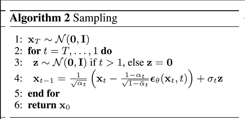DDPM paper: https://arxiv.org/abs/2006.11239

Training Algorithm#

Suppose that we have two multivariate normal distributions x and y, with means \(\mu_x\) and \(\mu_y\) and with (non-singular) covariance matrices \(\Sigma_x\), \(\Sigma_y\). If the two distributions have the same dimension, d, then the relative entropy between the distributions is as given below in equation 104. If you are interested, you can follow the proof here.

There is a KL divergence term in the loss function as shown in equation 70, which is the denoising matching term. Hence in our loss function, we want to optimize the KL divergence between the two distributions.

For our training purposes, we can set the variance for the two probability distributions to match to \(\Sigma_q(t) = \sigma^2_q(t) I\). In the DDPM, paper the authors decided to keep the variance fixed, and let the neural network only learn (represent) the mean \(\mu_\theta\) of this conditional probability distribution.

Using the relation for two multivariate normal distributions from equation 104 we can write as shown in equation 107 below.

The first term in equation 107 becomes log 1 hence we can cancel this. The third term is the trace function which resolves to d.

Resolving the variance term in equation 109 to \(\sigma^2_q(t) I\) gives results in equation 110. Then we can go to equation 111 because of the definition of the norm of two distributions.

Now we replace the values of \(\mu_q\) and \(\mu_\theta\), from the above equations 102 and 103. Then resolve the brackets by multiplying the terms with \(1/\sqrt{\alpha_t}\) and shown in equation 113. So, we can cancel out the \(x_t/\sqrt{\alpha_t}\) terms, leaving with us an equation with \(\epsilon_0\) and \(\epsilon_\theta\) terms as shown in 114.

Notice that the coefficients of both \(\epsilon_0\) and \(\epsilon_\theta\) terms are the same, so we can factor it out as shown in equation 115. If we take this outside the norm, that means we have to square the coefficient terms ie. \((1-\alpha_t)\) becomes \((1-\alpha_t)^2\) and the square roots in the denominators \(\sqrt{\alpha_t}\) and \(\sqrt{1-\bar{\alpha}_t}\) go away as shown in equation 116. Finally from equation 7, we replace the numerator with \(\beta_t\). We replace the \(x_t\) with the function of \(x_0\) and \(\epsilon_0\) from equation 20 showcasing the final form of the loss function as shown in equation 117.

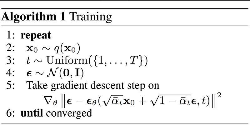source: DDPM paper https://arxiv.org/abs/2006.11239

Thus, we have derived the final form of the equation that is used in the training algorithm in the DDPM paper shown in the screenshot above. Here, \(\epsilon_\theta(x_t, t)\) is a neural network that learns to predict the source noise \(\epsilon_0 \sim \mathcal{N}(\epsilon; 0, I)\) that determines \(x_t\) from of \(x_0\).

Conclusion#

In this post we worked through the derivations of the sampling algorithm and the training algorithm as mentioned in the DDPM paper. For this we started with the definition of the forward and reverse diffusion and then worked through the ELBO method. If there is an part of the logic that is unclear or you think might not be correct, please reach out to me.

References and Further Reading#

1. Rogge, N. & Rasool, K. The Annotated Diffusion Model. HuggingFace Blog.
2. Adaloglou, N. How Diffusion Models Work: The Math From Scratch. The AI Summer.
3. Roy, S. A Beginner's Guide to Diffusion Models. Hashnode.
4. Song, Y. Generative Modeling by Estimating Gradients of the Data Distribution. 2021.
5. Stability AI. Stable Image.
6. MIT CSAIL. Flow Matching and Diffusion Models. Course website.
7. MIT. A Practical Introduction to Diffusion Models. YouTube playlist.
8. Fudan Generative Vision Lab. Diffusion GenAI Course. GitHub.
9. A Practical Introduction to Diffusion.
10. Gallon et al. An Overview of Diffusion Models for Generative Artificial Intelligence. arXiv:2412.01371.
11. Yang, C. Diffusion Models.
12. Deepia. Diffusion Models: DDPM. YouTube.
13. Chen et al. Comprehensive Exploration of Diffusion Models in Image Generation: A Survey. Springer, 2025.
14. Mehraban, S. Diffusion Models (DDPM & DDIM) — Easily Explained! YouTube.
15. Turc, J. The Physics Behind Diffusion Models. YouTube.
16. Deepia. Score-based Diffusion Models. YouTube.
17. Aggarwal et al. Generative Adversarial Network: An Overview of Theory and Applications. ScienceDirect.
18. Variational Autoencoders: How They Work and Why They Matter. DataCamp.
19. Wikipedia. Brownian Motion.
20. Winkler, L. Reverse Time Anderson.
21. Neal, R. M. Annealed Importance Sampling. arXiv.
22. Friedman, R. MCMC and Langevin Dynamics.
23. Wikipedia. Markov Chain Monte Carlo.
24. Wikipedia. Metropolis-adjusted Langevin Algorithm.
25. Gimenez, O. Bayesian Statistics and MCMC.
26. A Step by Step Tutorial on Diffusion. arXiv:2406.08929.
27. Das, A. Diffusion Probabilistic Models and their Connection to SDEs.
28. Guo et al. A Comprehensive Review on Noise Control of Diffusion Models. arXiv:2502.04669.
29. Turner et al. Denoising Diffusion Probabilistic Models in Six Simple Steps. arXiv:2402.04384.
30. Kim, J. Deriving Reverse-Time Stochastic Differential Equations.
31. Ghojogh et al. Factor Analysis, Probabilistic PCA, Variational Inference, and VAE: Tutorial and Survey. arXiv:2101.00734.
32. Jiang, Y. ELBO — Evidence Lower Bound.
33. Luo, C. Understanding Diffusion Models: A Unified Perspective. arXiv:2208.11970.
34. Stack Exchange. How is the variance for a diffusion kernel derived?
35. Stack Exchange. Expectation of sum is sum of expectations.
36. Stack Exchange. Integral of conditional probability density function.